Filtering a Random Loading Process in the Problem of Assessing the Durability of Rolling Stock Parts

Irina Gadolina^1,*, Aleksey Erpalov² and Kirill Khoroshevskii²

¹Institute of Mechanical Engineering RAS, Moscow, Russia
²South Ural State University, Chelyabinsk, Russia
E-mail: gadolina@mail.ru
*Corresponding Author

Received 28 October 2025; Accepted 25 November 2025

Abstract

The article addresses the urgent problem of selecting a filtering method for a random loading process, which in some cases may be non-stationary. This issue is closely related to the problem of durability assessment, as its solution determines how completely the oscillation components (including high-frequency ones) are represented in the output load vector. The problem is analysed using loading processes obtained from operational measurements of a real object at several commonly used movement speeds. Several filtering methods are analysed, including the use of low-frequency median filters, the level method, and modal decomposition. Since the processing involves subsequent durability assessment, conditional durability evaluations were performed to demonstrate the similarities and differences between the filtering methods in the calculations for the filtered processes. Recommendations for the preliminary processing of the data are provided.

Keywords: Random loading, rolling stock parts, filtration, durability assessment.

1 Introduction

There is a vast scientific literature devoted to the issues of filtering stationary, non-stationary, Gaussian and non-Gaussian processes. Let us focus on digital methods, without addressing analogue hardware techniques.

Previously, filtering issues were addressed in the development of forecasting methods, where eliminating random effects from the initial data and the studied processes was of significant importance [1]. The importance of considering random measurement errors was also noted. In the forecasted values, due to the above effects, a certain random background or “noise” is created. Filtering of noise should increase the reliability and justification of forecasts [1].

In [2], the filtering of non-stationary signals using the Kalman filter is considered. It is noted that if changes in the direction of movement of processes are detected at the time of receiving the current observation, then such detection is a forecast. The challenge lies in the fact that turning points are usually masked by the presence of short-period irregular random oscillations. Determining the moments of a trend or wave break is an important task for monitoring random processes.

In [3], attention is drawn to some ambiguity in establishing the boundary of narrow-band random processes. The use of filters with different bandwidths when constructing the envelope spectrum complicates the comparison of the obtained results in assessing the amplitude modulation depth in vibration diagnostics of defects in rotary machines. The results of band-pass filtering of the noise process, as well as amplitude-modulated noise, were studied.

An analysis of filtering results for a broadband normal random process with constant spectral density, where the spectrum width of the resulting oscillations is expressed through spectral moments, showed that processes isolated by a filter of no more than 1/3 octave should be considered narrow-band.

With regard to vehicles, the filtering of low-frequency random processes is considered in [4]. In the work, wave loads of the ship’s hull are considered as a linear dynamic system. It is noted that when passing through a linear stationary system, a normal random process remains normal. Averaging filters were employed to smooth low-frequency components.

Studies of random loading processes $σ$ (t), although they partially use the terminology adopted for processing random processes, have their own specifics. Thus, the rain flow method (refers to the methods of cycle counting, i.e. replacing a random loading process with a set of harmonics obtained according to special rules), recognized by scientists all over the world as the best, is used exclusively for processing random loading processes. The choice of the type of this algorithm (the method of full cycles, the method of paired swings, the method of hysteresis loops, etc.) has little effect on the essence of the matter and the result obtained. Optimal processing algorithms consider each implementation section sequentially once and can operate in the online process tracking mode. The rain flow method can be applied to loading in both the high-cycle and low-cycle regions [5, 6].

This article considers the actions to reject high-frequency oscillations. Also considered are the issues of choosing the implementation duration, choosing the number of quantization levels and determining the process irregularity coefficient I [6].

Methodological issues are illustrated using random loading processes obtained from strain gauge measurements of deformations in the structure of a diesel locomotive bogie frame. Recordings were made in the most loaded section of the bogie frame when moving along a straight section of track at different speeds.

The sequence of stages for processing a random loading process is as follows:

Estimate the required sampling frequency (based on earlier measurements);

Select the number of quantization levels (despite the almost limitless computational capabilities, it should not be excessively large);

Apply optimal filtering methods to reject high-frequency oscillations that may represent recording interference, and compare the results;

Identify extrema;

Identify full cycles using the rain flow method;

Compile a generalized block that reliably represents the expected operational history.

2 The Processes Under Study and Their Characteristics

For the methodological purposes of the study, three broadband random loading processes were selected, corresponding to different locomotive speeds: Vvel $=$ 80 km/h, s80; Vvel $=$ 70 km/h, s70; Vvel $=$ 60 km/h, s60. The stationarity hypothesis [7] was tested at a high level of statistical significance. The analysis results showed the following: (1) the s80 signal (80 km/h) can be considered stationary; (2) the s60 signal (60 km/h) exhibits non-stationary behaviour with a block size of about 100 samples: a trend is observed, as well as fluctuations in variance. However, when the block size is increased to 500 samples, the stationarity hypothesis is not rejected. With an intermediate block size (240 samples) and under the application of strict series test boundaries, the stationarity hypothesis is again rejected; (3) the s70 signal (70 km/h) is generally stationary, with one exception: with a block size of 240 samples, a deviation in the inversion criterion is observed, which may indicate the presence of a minor trend [7].

The shape of the probability density functions and their characteristics (asymmetry and excess), as well as deviations of the mode and median from the mean, refute the hypothesis of normality; in other words, the processes do not exhibit normal behaviour. The use of the rainflow cycle-counting method does not require fulfillment of the normality assumption, therefore, processes s80, s70 and s60 can be processed and the conditional fatigue life can be calculated.

Thus, the analysis confirms the feasibility of using the selected random processes for further research, despite their deviation from normality and partial non-stationarity in individual cases.

The statistical characteristics of the processes are presented in Table 1.

Table 1 The statistical characteristics of the processes

Characteristics of Empirical Probability Density	$s$ 80	$s$ 70	$s$ 60
Mean	−0.42	−3.33	−1.94
Standard error	0.08	0.07	0.07
Median	−0.88	−3.61	−1.98
Mode	−0.62	−7.13	−1.14
Standard deviation	7.92	7.01	7.19
Sample variance	62.75	49.16	51.73
Excess	−0.21	−0.24	−0.40
Asymmetry	0.23	0.21	0.19
Interval	51.17	49.15	44.57
Minimum	−22.04	−27.28	−22.35
Maximum	29.13	21.87	22.22
Amount	−4175.86	−32110.80	−18785.60
Account	10004	9638	9699

In [8], it is shown that due to the specific nature of the problems addressed in durability assessment, the sampling interval of random loading processes $Δ$ t should be chosen to be smaller than that recommended in the theory of random processes [7]. In [8], a formula is proposed, where $σ$ is the required relative accuracy of stress assessment; f is the maximum frequency of the process. Thus, the sampling step was estimated as $Δ$ t $=$ 0.004883 s. The stationarity requirements and conclusions based on them for random loading processes in the context of durability assessment are formulated somewhat differently than in [7]. For random loading processes, the concept of a “stationary random process in a special sense” was introduced in [9]. This concept is applicable exclusively to loading processes causing fatigue and describes the stabilization of calculated fatigue characteristics as the duration of measurements increases. The study [10] demonstrated that the implementations under consideration are stationary in a special sense. This means that a consistent durability assessment can be carried out based on the process data. For three processes moving at different speeds, the necessary and sufficient implementation length was estimated (Figure 1).

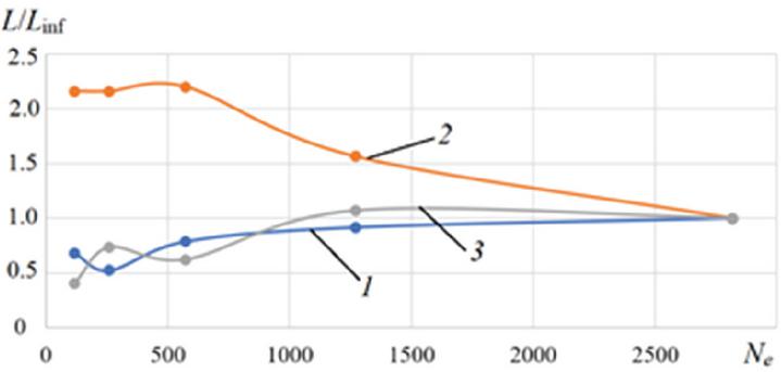
Figure 1 Estimation of the necessary and sufficient implementation length to obtain reliable durability estimates 1 – V $=$ 80 km/h; 2 – V $=$ 70 km/h; 3 – V $=$ 60 km/h.

Based on the graph (Figure 1), we can conclude that the length of the implementation Ne $=$ 2500 (Ne is the number of extrema with the number of quantization levels k $=$ 24) is sufficient for these implementations of the random processes. The rationale for this statement is that the fluctuations in the ratio L/L_inf, namely, the calculated resource L to the conditionally estimated resource on an infinite implementation L_inf, are insignificant and the ratio tends to unity. The values of the most important parameters for assessing the durability, such as the spectrum completeness parameter V(m) and the process irregularity coefficient I [6], also stabilize. The dependencies stabilize over time, which means that the processes are stationary in the special sense of durability assessment [9].

The spectrum completeness parameter V(m) is a value specific to durability assessment. When calculating this parameter, the linear hypothesis of damage accumulation and data on the coefficient of the slope of the fatigue curve m are used.

V(m) is calculated using the formula:

V = \sqrt[m]{\frac{1}{n} \sum h_{i} {(\frac{σ_{a i}}{{\hat{σ}}_{a}})}^{m}}

(1)

$σ_{ai}$ is the current value of the stress amplitude; hi is the number of cycles at the i-th stage; n is the total number of cycles in the block; $σ_{a}$ is the maximum amplitude in the block. This parameter also stabilizes with increasing implementation lengths for all three processes.

3 Filtration Methods

The study of random loading processes for the purpose of durability assessment has its own specifics. Therefore, the application of filtering methods should be considered taking into account that filtering serves as a preparatory stage for durability evaluation. Figure 2 shows a part of stress time histories of the loading process when a diesel locomotive is moving at speed of 80 km/h.

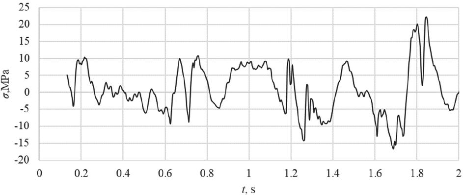
Figure 2 The part of realization of normal stresses acting in the frame structure when the diesel locomotive is moving at speed of 80 km/h.

A large number of low-amplitude, high-frequency oscillations can be observed. It is necessary to select and apply the optimal filtering method to reject high-frequency oscillations, which may be caused by recording or measurement interference. The optimal approach is to consider a physical model of the object generating the random loading process, taking into account information on its natural vibration modes, frequencies, and damping characteristics. In this case, the criterion for choosing the optimal filtering method will be the durability value obtained from calculations based on the filtered signal.

The spectral density graph S(f) of the original signal (Figure 3) shows that, for the unfiltered signal, the frequency range extends up to 25 Hz, which does not correspond to the operating frequency range of the supporting structures of the rolling stock. It was assumed that the high-frequency components represent interference from the measuring and recording equipment. This raises the question of selecting an appropriate method for high-frequency filtering.

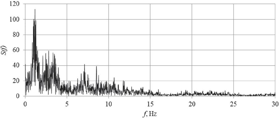
Figure 3 Power spectral density of the process V_vel $=$ 80 km/h.

Let us consider several filtering options, adapted to different extents to fatigue testing and calculations.

Low-pass median filters with different aperture sizes are examined. The median filter is one of the types of digital filters, widely used in digital signal and image processing to reduce noise levels. The median filter is a nonlinear filter [11, 12].

The sample values inside the filter window are sorted in ascending (descending) order; and the value in the middle of the sorted list is passed to the filter output. In the case of an even number of samples in the window, the filter output value is equal to the average value of two samples in the middle of the sorted list. The window then moves along the filtered signal and the calculations are repeated.

Median filtering is an effective method for processing signals affected by impulse noise. Median filters with aperture sizes of 5 and 9 are used for filtering. This means choosing the median value in a window with values of 5 and 9 samples. Large aperture values do not allow capturing significant extremes, which have a considerable effect on the calculated fatigue life. Figure 4 shows the initial section of the implementation of $V_{vel}$ $=$ 80 km/h at the output of the median filter with an aperture of 5.

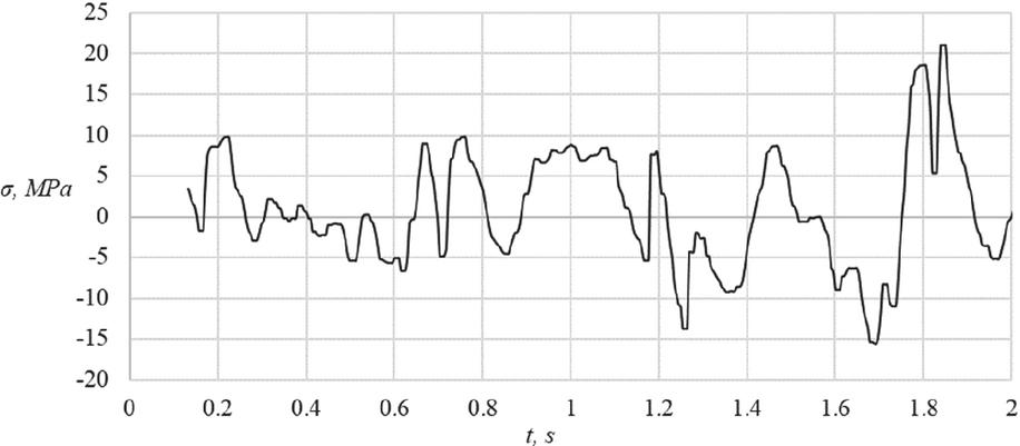
Figure 4 The beginning of the process Vvel $=$ 80 km/h, filtered using median filters, aperture 5.

Compared to the original implementation (Figure 2), this example demonstrates that high-frequency oscillations are eliminated by filtering. Next, we compare the filtered data using the median filter method with different aperture sizes: 5 and 9. For an aperture of 9, the filtered processes for all three investigated processes turned out to be less damaging (i.e., the calculated durability will be greater, since the points of significant local extrema of the implementation were missed). Therefore, an aperture of 5 was chosen for further calculations.

Filtering by the level method. Frequency filtering is not the only way to reject low-amplitude oscillations in the digital processing of random loading processes. GOST [6] recommends the use of the level method. The essence of the method lies in dividing the process implementation into classes vertically – quantization. Samples of the discretized implementation that fall into one class are considered as one sample. Using this algorithm, it is also possible to isolate local process extremes while saving computational resources. The algorithm was previously used especially effectively in analogue devices [13]. In digital processing, the method is applied in three stages: (1) a horizontal grid of levels is superimposed on the discretized sequence. According to [6], the number of levels can vary from 12 to 36. The grid is constructed to include the maximum and minimum values of the implementation; (2) a sequence of samples is considered and sub-sequences that fall into one class are discarded. In this case, information about the frequency composition is lost, since it is assumed that the most critical information is contained in the values of the extremes; (3) extremes are highlighted.

Filtering using empirical mode decomposition (EMD) and variational mode decomposition (VMD). In [14], a new method for assessing the durability of structures is proposed, based on the application of an adaptive variational mode decomposition method to signals from sensors, including non-stationary ones. As a result of the decomposition, narrow-band signals of a simple structure are obtained, which are then processed using the rain-flow method in the time domain [6]. It is proposed to consider a non-stationary random process as a composition of stationary ones. In this article, as well as in [15–17], the EMD and VMD decomposition methods are used. These methods are used to filter a random process, by removing high-frequency oscillations. The EMD method consists of decomposing a signal x(t) of length Lx into a set of M empirical modes (internal oscillations). After the decomposition, a remainder r is isolated, which corresponds to the general trend of the process [18]. Figure 5 shows: (a) the beginning of the initial recording of stresses in the bogie frame element at a speed of 60 km/h; (b) the filtered signal using EMD. It is evident that the small-amplitude oscillations disappear after filtering.

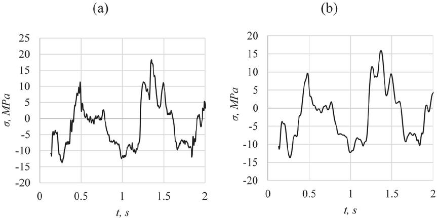
Figure 5 Original process (a) and filtered process using EMD (b).

Advantages of using EMD [14] for filtering signals: (1) adaptivity – does not require specifying the modes into which decomposition occurs; (2) only the first mode is “thrown out” as the highest-frequency (it is assumed that the noise in the signal has a high-frequency nature); (3) if necessary, it is possible to eliminate a nonlinear trend in the signal.

The disadvantage of EMD is that the method does not always distinguish modes well – for individual signals it may not filter the signal correctly (checking is necessary).

The VMD method [18] has some advantages over EMD, namely, it is a fully adaptive and non-recursive algorithm for time-frequency signal analysis. The main hypothesis of the method is the assumption that any original signal can be decomposed into a finite number of modes that have different central frequencies and limited bandwidths.

4 Study of the Process Irregularity Coefficient I and the Spectrum Fullness Coefficient V(m) when Filtering Using Different Methods

The irregularity coefficient I (in signal processing problems it is called the broadband parameter) is an informative indicator of the complexity of the process structure [3, 6]:

I = \frac{N_{0}}{N_{e}}

(2)

Where N₀ and N_e are the numbers are the numbers of intersections of the average level and the number of extremes, respectively, calculated for a representative segment of the implementation.

Figure 6 shows the dependence of the calculated coefficient of irregularity of the process I on the number of levels of the intervals of change of the random process.

Figure 6 Calculated coefficient of irregularity I for three processes with a change in the number of levels: 1 – Vvel $=$ 60 km/h; 2 – Vvel $=$ 70 km/h; 3 – Vvel $=$ 80 km/h.

It is evident that coefficient I increases with decreasing number of levels. This means that this coefficient strongly depends on the number of quantization levels (which is a subjective choice of the researcher) and, therefore, cannot serve as a robust characteristic of the process [19]. Nevertheless, it is actively used in methods of durability assessment in the frequency domain [20]. This feature should not be overlooked when calculating durability in the frequency domain. Tables 2 and 3, as well as Figure 6, show the parameters of processing the filtered signals obtained on the basis of the implementation of Vvel $=$ 80 km/h and the implementation of Vvel $=$ 60 km/h. In the tables: Sa max, MPa – maximum amplitude in the block of amplitudes, selected using the rain-flow method [5, 6]; V(m) – coefficient of spectrum fullness, formula (1); I – coefficient of process irregularity, formula (2).

Table 2 Maximum amplitudes of filtered spectra, spectrum fullness coefficient V(m $=$ 5) and irregularity parameter I for the implementation of Vvel $=$ 80 km/h

		Median	Level Method	Filtering	Filtering
		Filters	(32 Classes/	Using	Using
	No Filtering	Aperture 5	16 Classes)	EMD	VMD
$S_{a \max}$ , MPa	23.52	23.47	23.63/23.88	23.52	25.67
$V_{(m = 5)}$	0.37	0.45	0.42/0.45	0.45	0.36
$I$	0.20	0.43	0.34/0.42	0.40	0.17

Table 3 Maximum amplitudes of filtered spectra, spectrum fullness coefficient V(m $=$ 5) and irregularity coefficient I for the implementation of Vvel $=$ 60 km/h

		Median	Level Method	Filtering	Filtering
		Filters	(32 Classes/	Using	Using
	No Filtering	Aperture 5	16 Classes)	EMD	VMD
$S_{a \max}$ , MPa	21.01	20.79	20.84/23.88	21.42	22.23
$V_{(m = 5)}$	0.39	0.45	0.44/0.45	0.39	0.37
$I$	0.16	0.46	0.32/0.37	0.40	0.15

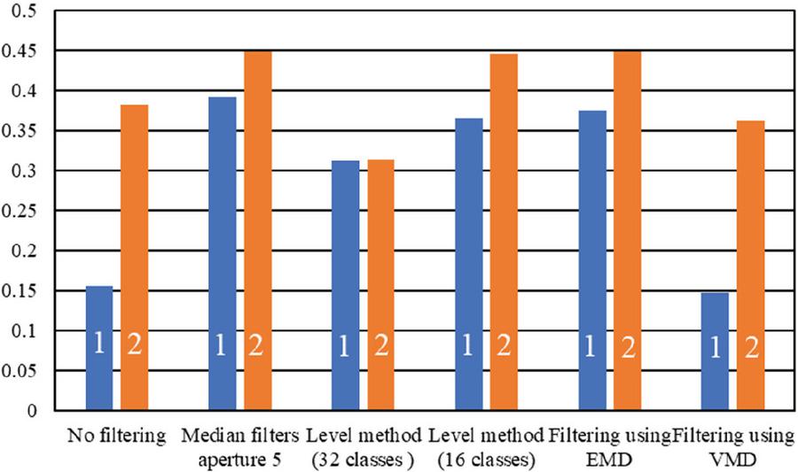
Figure 7 Characteristics of the loading process Vvel $=$ 60 km/h using different filtration methods: 1 – I; 2 – V(m).

Comparing the data in the tables and examining Figure 7, it can be seen that, according to these indicators, VMD filtering yields results close to the original signal, while the results of other methods are approximately the same. For the processes V_vel $=$ 70 km/h and V_vel $=$ 80 km/h, the nature of the dependencies was similar to the dependencies shown in Figure 7.

5 Comparison of the Obtained Results for Filtering. Comparison of Histograms

Since the present study is aimed at refining the calculated assessment of durability, when comparing the filtering methods, emphasis was placed on the indicators associated mainly with this area of research.

The histograms of the distributions of the amplitudes of complete cycles for the original and processes filtered by different methods differ in shape and in the magnitude of the maximum amplitude. The unfiltered signal contains many oscillations with minimal amplitude. Although damage from load oscillations with a small amplitude is significantly less than from oscillations with a significant load, their large number in the total cannot but have an effect. In Figure 8 shows the histograms of the distribution of the amplitudes Sa of the full cycles of the process V_vel $=$ 60 km/h.

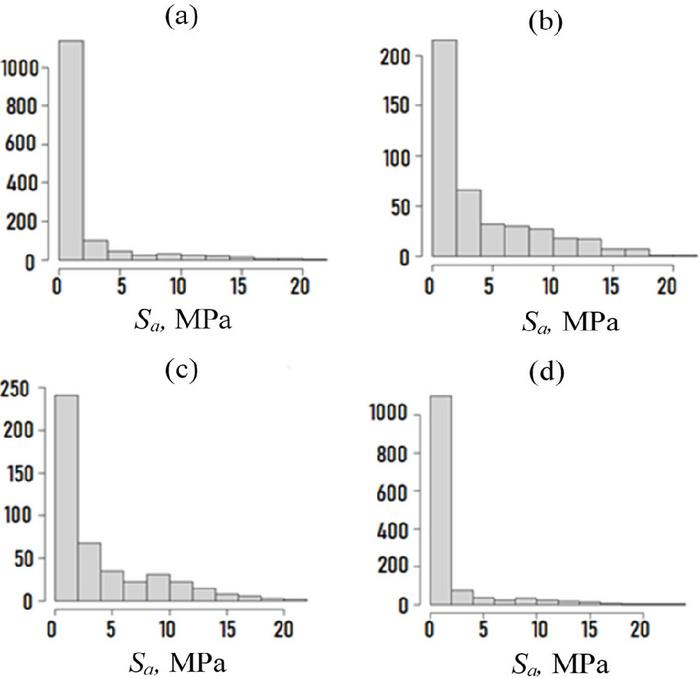
Figure 8 Histograms of the distribution of the amplitudes of full cycles of the process Vvel $=$ 60 km/h for the original process and for processes filtered by different methods: (a) – original process; (b) – median filters; (c) – EMD filtering; (d) – VMD filtering.

Changing the frequency composition of processes. Filtering processes reduces the recorded number of process extremes and the number of intersections of the average level f0. We define this indicator as

f_{0} = \frac{N_{0}}{t (l_{b})}

(3)

where t(l_b) is the time, it takes the train to pass l_b – loading block.

Figure 9 shows the frequencies of intersections of three processes of average levels per second when filtering using the intersection method for three variants of process filtering.

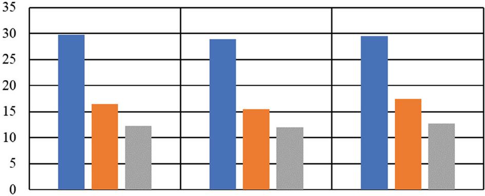
Figure 9 Frequency of crossings of the average level f0 when filtering by levels depending on the number of levels: blue– without filtering; brown – filtered by the level method with 32 levels; grey – filtered by the level method with 16 levels.

Comparison of conditional durability estimated by filtering using different methods.

Since the objective of this study is to estimate durability, the criterion for comparing the filtering methods was the estimated durability. The researchers did not have any experimental data on the fatigue characteristics of the complex structural element (bogie frame), so the calculation of fatigue damage was performed in conditional values. The processes were pre-filtered, and then the rain flow method was applied to them. The full cycles identified by the rain method (Figure 8) were used to calculate the conditional durability L using formula (4). The conditional durability was calculated for comparison with the results obtained using other filtering methods. The coefficient of the slope of the fatigue curve for the part was estimated to be m $=$ 5, which was used in the calculation [21]:

L = D^{- 1} l_{b}

(4)

where l_b is the loading block, the value in relation to which the durability is estimated, km; D is the damage per block, calculated in general terms according to the linear hypothesis using formula (5) [21].

D = K \sum_{i = 1}^{M} r_{a i}^{m} r_{a}

(5)

where K is a coefficient depending on the fatigue resistance properties of the part, rai are the amplitudes of the full cycles identified by the rainflow method. Summation is performed over all M cycles in the implementation. By setting an arbitrary coefficient K using formulas (4) and (5), we obtain the so-called conditional durability. Figure 8 shows for comparison the calculated conditional durability for the bogie frame element at different speeds when filtering processes by different methods. The closest to the original implementation indicators for the calculated durability were obtained when filtering by the VMD method. The greatest durability was obtained when filtering by the median filter method. Perhaps this is due to the fact that this method filters the process most radically. Also, filtering by the level method with 16 levels gives relatively close results for the calculated durability, compared to the results obtained for the implementation before filtering.

This does not mean that filtering by this method is optimal, since the filtering goal may not be achieved, namely, reducing the number of extremes for testing. Note that for a speed of 80 km/h, the conditional durability is lower, since the vibrations at high speed are higher and the damage D from formula (5) is correspondingly higher. The durability for the speeds of V_vel $=$ 60 km/h and V_vel $=$ 70 km/h for all filtering methods almost coincide.

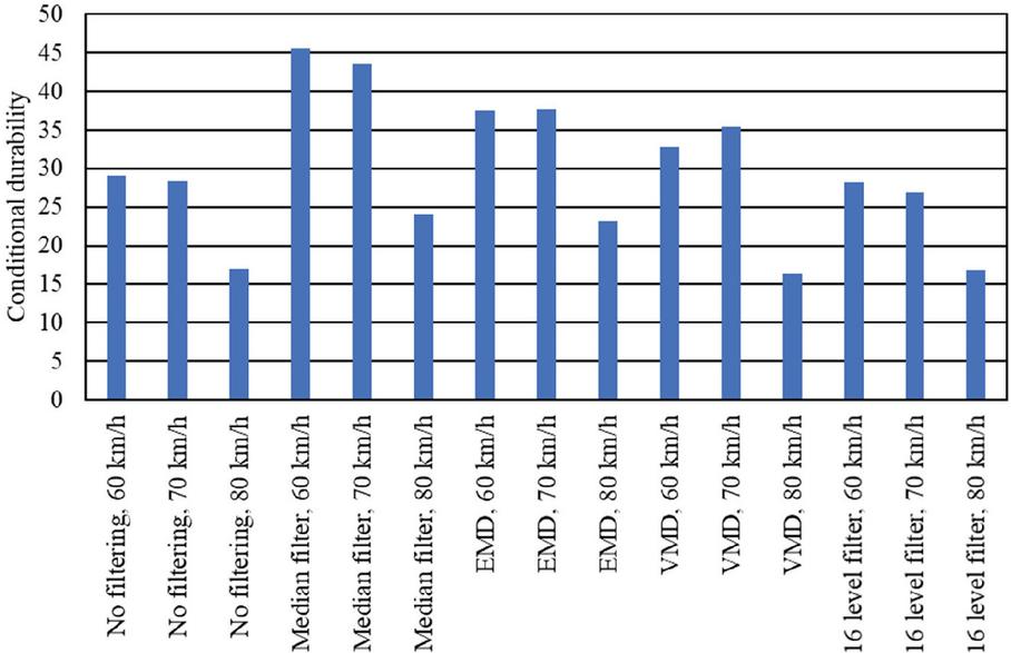
Figure 10 Conditional durability of a part when moving at different speeds with filtering by different methods.

6 Discussion

(i) Several filtering methods are considered, such as the empirical mode decomposition method EMD and the variational mode decomposition VMD. The analysis by different methods is carried out both in the time and frequency domains. Since the filtering methods are considered here as a preparatory stage for the durability assessment, the comparison of methods is performed based on the calculated values of conditional durability. The comparison showed that filtering by median filters (the highest durability) and by the level method with 16 levels (the lowest durability) form a kind of “fork” inside which other results on the calculated durability are located.

(ii) Specific issues related to the processing of load processes are analysed, such as determining the necessary and sufficient implementation length, the number of quantization levels, the spectrum fullness parameter V(m).

(iii) After filtering by the described methods, the frequency band of the three filtered processes was 7–12 Hz. The processes are similar in structure before and after filtering. For the process V_vel $=$ 80 km/h, some excess in relative damage was recorded and, accordingly, the conditional durability was lower. The irregularity coefficient I strongly depends on the number of quantization levels and therefore cannot serve as an invariant characteristic of a random loading process. The final conclusion on the advantages of one or another filtering method can be made after conducting a fatigue experiment to assess the lower damaging limit of stress amplitudes.

7 Conclusion

• To solve the actual problem of choosing the optimal filtering method, a number of previously used filtering methods, as well as two new methods based on signal decomposition, were analysed using examples of operating modes in a rolling stock part.

• It was noted that the problem of choosing how to reject low-amplitude oscillations is closely related to determining the threshold of damaging amplitudes. The latter requires additional experimental study.

• The efficiency of the filtering methods was estimated by the durability calculated from filtered processes during schematization using the rain-flow method and estimating the conditional durability using the linear damage summation hypothesis.

• It was shown that all the considered filtering methods can be used in engineering applications of durability assessment, as well as in testing. The VMD (variational mode decomposition) and EMD (empirical mode decomposition) methods combine the principles of frequency and time analysis, which makes them suitable for solving the engineering problem of fatigue assessment and testing.

Funding

The study was supported by the grant of the Russian Science Foundation No. 25-29-20268, https://rscf.ru/project/25-29-20268/.

References

[1] Valishin, A. A., Zaprivoda, A.V., Klonov, A. S. (2024) Mathematical modeling and comparative analysis of numerical methods for solving the problem of continuous discrete filtering of random processes in real time. Mathematical modeling and numerical methods. No. 1(41). pp. 93–109. DOI: 10.18698/2309-3684-2024-1-93109.

[2] Grebenyuk, E. A. (2013) Filtering of non-stationary signals using the Kalman filter in the task of monitoring non–stationary processes/E. A. Grebenyuk. Management of the development of large-scale systems (MLSD’2013): Proceedings of the Seventh International Conference: in 2 volumes, Moscow, September 30–02/Institute of Management Problems RAS; under the general editorship of S.N. Vasiliev, A.D. Tsvirkun. Volume II. Moscow: Trapeznikov Institute of Management Problems of the Russian Academy of Sciences. pp. 439–446.

[3] Sundukov, A. E. (2020) Substantiation of the choice of filter width when using the envelope spectrum in vibration diagnostics of defects in rotary machines Bulletin of the Samara University. Aerospace engineering, technology, and mechanical engineering. Vol. 19, No. 3. pp. 100–108. DOI: 10.18287/2541-7533-2020-19-3-100-108. – EDN BAKKAD.

[4] Korolev, V. V., Zhadobin, N. E., Zastavny, S. V. (2009) Filtering of low-frequency random processes occurring in the ship’s hull. Operation of marine transport. No. 1(55). pp. 65–67.

[5] Kogaev, V.P. (1993) Calculations for strength under stresses of variables over time. Moscow, Mashinostroenie. 364 p.

[6] GOST 25.101-83. (2005) Calculations and strength tests. Methods of schematization of random processes of loading of machine elements and structures and statistical representation of the results. Moscow. Standartinform, 25 pages

[7] Bendat, Julius S., Piersol, Allan G. (2011) Random data. A timely update of the classic book on the theory and application of random data analysis. A Wiley-Interscience Publication. John Wiley & Sons. New York Chichester.

[8] Gadolina, I. V., Lisachenko, N. G., Svirskiy, Y. A., Dubin, D. A. (2020) The Choice of Sampling Frequency and Optimal Method of Signals Digital Processing in Problems of a Random Loading Process Treating to Assess Durability. Inorganic Materials. Vol. 56, No. 15. pp. 1551–1558. DOI: 10.1134/S0020168520150054. – EDN CMXMNY.

[9] Gadolina, I. V. (2024) Evaluation of the optimal length of realization of random loading in the study of the durability of machine parts. Reliability. Vol. 24, No. 1. pp. 51–57. DOI: 10.21683/1729-2646-2024-24-1-51-57.

[10] Gadolina, I.V., Gasyuk A.S., Erpalov A.V. (2024) Investigation of the stability of a random loading process using a spectral and temporal approach. Proceedings of the 7th International Scientific and Technical Conference “Survivability and structural Materials Science” ZHIVKOM, pp. 202–207.

[11] Tukey, J.W. (1971) Exploratory Data Analysis. Addison - Wesley, Reading, Mass.

[12] Bolshakov, I.A., Rakoshits, V.S. Applied Theory of Random Flows, Moscow. Soviet Radio, 1978, 248p.

[13] Description of the invention to the copyright certificate 1322161. (1986) A device for determining the extremes of an electrical signal. Institute of Technical Heat Engineering of the National Academy of Sciences of Ukraine. Kiev.

[14] Erpalov, A. V., Khoroshevsky, K. A., Rumyantseva, E. A., Gadolina I. V. (2024) A method for assessing the durability of structures under stationary and non-stationary random loads using variational mode decomposition. Industrial Laboratory. Diagnostics of Materials. Vol. 90, No. 9. pp. 63–74. DOI: 10.26896/1028-6861-2024-90-9-63-74.

[15] Jae Yoon (2018) A novel approach for stress cycle analysis based on empirical mode decomposition. MFPT. Intell. Technol. Equip. Hum. Perform. Monit. Proc. pp. 4–12.

[16] Fu J., et al. (2020) An Improved VMD-Based Denoising Method for Time Domain Load Signal Combining Wavelet with Singular Spectrum Analysis. Math. Probl. Eng. Vol. 2020.1485937. DOI: 10.1155/2020/1485937.

[17] Soman, R. (2020) Semi-automated methodology for damage assessment of a scaled wind turbine tripod using enhanced empirical mode decomposition and statistical analysis. Int. J. Fatigue. Vol. 134. 105475. DOI: 10.1016/j.ijfatigue.2020.105475.

[18] Dragomiretskiy, K., Zocco, D. (2014) Variational Mode decomposition. IEEE Trans. Signal Process. Vol. 62. No. 3. pp. 531–544. DOI: 10.1109/TSP/2013.2288675.

[19] Gadolina, I. V., Petrova, I. M., Dubin, D. A., Serebriakova, I. L. (2020) Stabilization of the Design Loading Characteristics in the Problems of Durability Estimation of Tracked Vehicle Parts. Journal of Machinery Manufacture and Reliability. Vol. 49, No. 1. pp. 31–37. DOI: 10.3103/S1052618820010069.

[20] Dirlik, T., Benasciutti, (2021) D. Dirlik and Tovo-Benasciutti Spectral Methods in Vibration Fatigue: A Review with a Historical Perspective / Metals (Basel). Vol. 11, No. 9. pp. 1333–1345.

[21] Dreßler, K., Speckert, M., Müller, R., Weber, Ch. (2009) Customer loads correlation in truck engineering. Berichte des Fraunhofer ITWM, Nr. 151.

Biographies

Irina Gadolina received the master’s degree in mechanical engineering from Bauman Moscow State Technical University in 1977, and the philosophy of doctorate degree in Mechanical Engineering Research Institute of the Russian Academy of Sciences in 1990, respectively. She is currently working as a Senior Research worker in Mechanical Engineering Research Institute at the Department of Structural Materials Science. Her research areas include random loading professes investigation, metal fatigue analysis. She has been serving as a reviewer for some highly-respected journals.

Aleksey Erpalov received the master’s degree in mechanical engineering from South Ural State University in 2012 and and the philosophy of doctorate degree in South Ural State University in 2017, respectively. He is currently working as Deputy Director of Center of Vibration Testing and Monitoring Structural Components. His research areas include vibration strength, service life of structures, fatigue testing, experimental studies of the strength properties of structures, dynamic testing.

Kirill Khoroshevskii received the bachelor’s and master’s degree in Rocket Engineering from South Ural State University in 2019 and 2021 correspondingly. He is currently working as an engineer in Center of Vibration Testing and Monitoring Structural Components.