Mathematical Modelling: Transforming Concepts Into Reality

Simran Sahlot and Geeta Arora^*

Department of Mathematics, Lovely Professional University, Punjab, India
E-mail:
*Corresponding Author

Received 19 October 2024; Accepted 22 December 2024

Abstract

Mathematical modelling is a powerful tool that bridges the gap between theoretical concepts and real-world phenomena. It involves the development of mathematical equations, algorithms, and computational techniques to describe, analyse, and predict complex systems across various disciplines. Researchers are creating mathematical models based on actual events to meet the demands of this scientific era. The main aim of mathematical modelling is to gain understanding into complex systems, make predictions, and optimize processes. By using mathematical equations, scientists and researchers can simulate and analyse various scenarios, explore the effects of different parameters, and make informed decisions. Mathematical models can provide a better understanding of the given mechanisms governing the system and help uncover relationships and patterns that may not be immediately apparent. Policymakers use mathematical models to inform their choices when deciding on public health interventions like lockdowns, social isolation tactics, and vaccination rollout plans.

Keywords: Mathematical modelling, computational techniques, social isolation tactics.

1 Introduction

The process of representing real-world phenomena or systems using mathematical actions, formulas, or algorithms is called mathematical modelling. It is a way to describe, analyse, and predict the behaviour of complex systems or processes by translating them into a mathematical framework. It is used in a wide range of areas including engineering, biology, physics, economics, and social sciences. By creating mathematical models, researchers can simulate and predict the behaviour of complex systems, test hypotheses, and gain insights into the underlying mechanisms as shown in Figure 1. Mathematical modelling involves constructing a set of equations that shows the behaviour of a system, and then solving those equations to predict system behaviour under different conditions. This allows researchers to explore the effects of changing variables and parameters on the system, and to identify optimal solutions or strategies [1]. Mathematical modelling has many practical applications, from designing new technologies to predicting the spread of diseases, and it continues to be an important area of research in many fields [2].

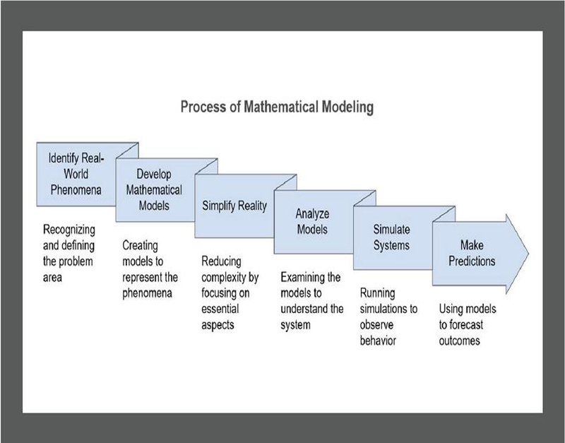
Figure 1 Process of mathematical modelling.

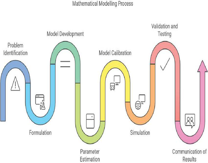
Figure 2 Steps involved in the formulation of mathematical model.

1.1 Steps Involved in Mathematical Modelling

The mathematical modelling process follows an organized approach, starting with Problem Identification in which the problem requires to explore through mathematical approaches is clearly defined. After that in Formulation the relevant variables, parameters, and relations are identified and represented using equations or functions. The model is simplified by providing logical assumptions on the system, defining its application and boundaries. After that the data is collected from experiments, observations, or existing sources to ease estimation and validation. After creating the structure, Model Development takes place, generating a mathematical representation using defined equations and assumptions including differential equations, statistical models, or optimization methods. In Parameter Estimation, the values of unknown parameters are derived from existing data which frequently uses approach to estimate the probability. Model calibration modifies these parameters to ensure compatibility with observed data, thus enhancing the precision of the model. By using the validated model, simulations are performed to predict system behaviour which enables sensitivity evaluations and providing understanding of the dynamics of the system under various circumstances. The reliability and precision of the model are evaluated during the Validation and Testing phase by comparing predictions with independent data or real-world observations. All required modifications are implemented according to these assessments as shown in Figure 2. Finally, the Communication of Results is important as it conveys results, and model limitations to researchers by including detailed explanation of assumptions, methodologies, and interpretations [3].

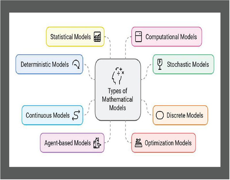
Figure 3 These are few types of mathematical modelling.

1.2 Types of Mathematical Modelling

There are several important types of mathematical modelling used in various fields as shown in Figure 3. Here are some of the key types:

1.2.1 Deterministic models

These models use mathematical equations to represent relationships between variables. They aim to predict outcomes with certainty by assuming inputs are known precisely. One of the well-known deterministic model is Euler’s model [4]. It is a simple numerical approach to solve ordinary differential equations (ODEs) with a given initial condition. It predicts the solution by frequently moving from an initial position along a tangent line in small increments, believing that the slope of the function remains constant throughout these increments [5]. Considering the differential equation:

\frac{d y}{d x} = f (x, y)

with an initial condition $y (x_{0}) = y_{0}$ . Euler’s method aims to approximate $y (x)$ over a specified interval by stepping forward from $x_{0}$ using a small step size $h$ . The formula for Euler’s method is:

y_{n + 1} = y_{n} + h \cdot f (x_{n}, y_{n})

where:

• $y_{n}$ is the approximate value of $y$ at $x_{n}$ ,

• $h$ is the step size,

• $f (x_{n}, y_{n})$ is the slope at $(x_{n}, y_{n})$ .

Euler’s approach has been applied in several fields. In physics, it helps to model motion, thermodynamics, and wave propagation. The approach enables the simulation of systems controlled by differential equations including control systems and circuit analysis. Euler’s approach is utilised in economics to address dynamic models in macroeconomics, primarily those related to capital accumulation [6].

A key advantage of Euler’s approach is its simplicity. The technique is simple to create and demands low computing power making it suitable for educational applications and for addressing situations where high precision is not required. Also, it offers an essential understanding of numerical methods by serving as a starting point to more advanced approaches such as Runge-Kutta methods [7].

1.2.2 Stochastic models

Stochastic models take into account randomness and uncertainty in the system being modelled. They use probability distributions and statistical methods to represent the variability in the data or processes. Example includes Markov chains [8]. Markov chains are systems that define the transition from one state to another in a sequential way. They are used in several domains, including finance, biology, and computer science, to model stochastic systems wherein the result of a process relies entirely on the current state, independent of any previous states. The memoryless characteristic is known as Markov property [9]. The Markov chain consists of:

• States: Distinct possible conditions the system can be in.

• Transition Probabilities: The probability of transfering from one state to another.

For Markov chain with states $S = {s_{1}, s_{2}, \dots, s_{n}}$ , the transition probability from state $s_{i}$ to state $s_{j}$ is shown by $P (s_{j} | s_{i})$ . The matrix containing all these transition probabilities is known as the transition matrix $P$ .

Transition Matrix The transition matrix $P$ for Markov chain with $n$ states is an $n \times n$ matrix, where each entry $P_{i j}$ represents the probability of transitioning from state $s_{i}$ to state $s_{j}$ :

P = [\begin{matrix} P_{11} & P_{12} & \dots & P_{1 n} \\ P_{21} & P_{22} & \dots & P_{2 n} \\ ⋮ & ⋮ & ⋱ & ⋮ \\ P_{n 1} & P_{n 2} & \dots & P_{n n} \end{matrix}]

Each row of $P$ sums to 1 since they represent probabilities of moving from one state to all possible states. Markov chains are widely used in modelling systems where future states depend only on the present state making them ideal for predicting sequential events in areas like finance, weather forecasting, and genetics. Their ability to capture dependencies in random processes is crucial in queueing theory for optimizing service systems and in web page ranking algorithms, like Google’s pagerank. They are also effective in reliability analysis for estimating the life of systems [10]. Advantages of Markov chains include their mathematical simplicity, ability to model stochastic processes, and adaptability for both theoretical studies and practical applications across diverse fields.

1.2.3 Discrete models

Discrete models are used when the system being modelled changes in distinct steps or events rather than continuously. They deal with countable and finite elements or states [11]. Example includes finite element analysis. The finite element analysis model is a robust computational tool for tackling complex engineering and mathematics challenges especially those are related to physical phenomena such as structural analysis, heat transfer, and electromagnetism. Finite element analysis decomposes a significant complex problem into smaller more manageable elements known as finite elements. The solutions of these distinct components are subsequently combined to produce an approximate solution for the entire system. The general formula for FEA can be expressed as:

KU = F

where, K: Global stiffness matrix, representing the system’s resistance to deformation (or generalized stiffness in other physics-based contexts). U: Vector of nodal unknowns (e.g., displacements in structural analysis, temperatures in thermal analysis). F: Global force vector (or load vector) representing external forces, heat sources, or other applied influences. Finite element analysis offers advantages, including its versatility to handle complex geometries, materials, and loading situations effortlessly. The precision yields complete data, especially with a finer mesh detail, ensuring correct evaluations. Also, its versatility enables it to tackle a broad spectrum of physical issues by changing governing equations and boundary conditions. Its application lies in structural engineering, it assesses stress, strain, and displacement in structures such as beams, frames, and buildings in mechanical engineering, it helps the design and analysis of components subjected to stress and dynamic loads. The aerospace sector use finite element analysis to evaluate material performance under severe conditions whereas in biomedical engineering it simulates the stress distribution in artificial joint and human tissues. It is essential for thermal analysis to solve heat transfer problems in electronic devices and various systems [12].

1.2.4 Continuous models

Continuous models are used when the system being modelled changes smoothly over time or space. They involve functions and equations defined on continuous domains [13]. Examples include fluid dynamics models. Fluid dynamics models describe the behavior of fluid flow (liquids and gases) and are essential in fields such as engineering, meteorology, oceanography, and physics. They are typically governed by the Navier-Stokes equations, which express the conservation of mass, momentum, and energy in a fluid [14]. The fundamental equations of fluid dynamics are derived from Newton’s second law which is applied to fluid motion, and can be expressed as:

ρ (\frac{\partial u}{\partial t} + (u \cdot \nabla) u) = - \nabla p + μ \nabla^{2} u + f

where:

• $ρ$ is the fluid density,

• $u$ is the fluid velocity vector,

• $p$ is the pressure,

• $μ$ is the dynamic viscosity,

• $f$ is the external force applied to the fluid.

These equations represent:

• Conservation of Mass: Often expressed as the continuity equation, ensuring that fluid mass is conserved.

• Conservation of Momentum: Describes the forces acting on fluid particles due to pressure, viscosity, and external forces.

Fluid dynamics models are widely applied across various fields. In engineering as they are essential for designing fluid systems such as pipelines, ventilation networks, and aircraft. Meteorology and oceanography depend upon these models to simulate atmospheric and ocean currents for weather forecasting. In biology, fluid dynamics aids in understanding blood flow in the cardiovascular system and airflow in respiratory systems. Environmental science uses these models to predict the dispersion of pollutants in air and water [15]. The strengths of fluid dynamics models include their predictive power for simulating complex behaviors like turbulence and vortices, versatility across different scales from microscopic to large-scale applications, and flexibility in adapting to factors like temperature, pressure, and external forces allowing for broad real-world applicability.

1.2.5 Agent-based models

Agent-based models simulate the behaviour of individual agents or entities and their interactions within a system. These models are particularly useful for studying complex systems with emergent properties [16]. Example includes social network models. Social network models are mathematical frameworks that analyse relationships and interactions among individuals within a social structure. In these models nodes represent participants while edges denote the connections between them, such as friendships or collaborations. The relationships can be represented using an adjacency matrix $A$ , where

A_{i j} = {\begin{matrix} 1 & if there is a connection between nodes i and j \\ 0 & otherwise \end{matrix}

Key metrics, like the degree of a node which counts the number of direct connections can be calculated as:

d_{i} = \sum_{j = 1}^{n} A_{i j}

where $d_{i}$ is the degree of node $i$ and $n$ is the total number of nodes. Also, betweenness centrality quantifies a node’s role in facilitating communication between other nodes expressed as:

C_{B} (i) = \sum_{j \neq i \neq k} \frac{σ_{j k} (i)}{σ_{j k}}

where $σ_{j k}$ is the total number of shortest paths from node $j$ to node $k$ , and $σ_{j k} (i)$ is the number of those paths that pass through node $i$ . These models can also utilize metrics such as graph density $D$ , which measures how interconnected a network is:

D = \frac{2 E}{N (N - 1)}

where $E$ is the number of edges and $N$ is the number of nodes. Models like pagerank can determine the importance of nodes based on their connectivity, computed as:

P R (i) = (1 - d) + d \sum_{j \in M (i)} \frac{P R (j)}{C (j)}

where $M (i)$ is the set of nodes that link to $i$ , $C (j)$ is the number of links from node $j$ , and $d$ is a damping factor. These social network models find applications in various fields, including information diffusion, community detection, and influence propagation, offering valuable insights into social dynamics. Their strengths lie in their ability to visually represent complex relationships by providing quantitative measures for analysis, and adapt to evolving social processes making them valuable tools for understanding the problems in human interaction [17].

1.2.6 Optimization models

Optimization models aim to find the best solution or set of solutions that optimize a specific objective function while satisfying a set of constraints. These models are widely used in operations research, logistics, and decision-making processes [18]. Example includes multi objective optimization model. The multi objective optimization model is formulated to address challenges with many frequently conflicting objectives, trying to find a collection of optimal choices among these objectives rather of a singular ideal solution. In these models, decision-makers pursue a collection of optimal solutions where strengthening one objective results in a loss of another. In a multi objective optimization problem, the goal is to optimize multiple conflicting objectives simultaneously, formulated as:

Minimize F (x) = [f_{1} (x), f_{2} (x), \dots, f_{k} (x)]

subject to:

g_{j} (x) \leq 0, j = 1, 2, \dots, m

h_{l} (x) = 0, l = 1, 2, \dots, p

x \in S

where $F (x)$ is the vector of $k$ objectives, and $g_{j} (x)$ and $h_{l} (x)$ define the feasible region $S$ . Multi objective optimization models are crucial for solving complex decision-making situations that need to resolve of several conflicting objectives. They allow decision-makers to assess decisions among objectives, making them particularly relevant in fields such as supply chain management (where cost, delivery time, and environmental impact require balance), engineering design (to enhance performance, cost, and safety), energy management (to reconcile reliability, cost, and sustainability), and finance (to optimize risk in relation to return). These models provide a collection of optimal choices, allowing decision-makers to choose solutions according to their priority. Multi objective optimization provides flexibility for handling conflicting objectives, robustness in revealing alternatives, and changes across many industries requiring complex decision-making. This method allows stakeholders to make wise choices that align with various organizational or strategic goals [19].

1.2.7 Statistical models

Statistical models use statistical techniques to describe and analyse data, identify patterns, and make predictions. These models often involve estimating parameters based on observed data and making inferences about the population [20]. Example includes Bayesian models. A Bayesian model is a statistical structure that employs Bayesian estimation to adjust the probability of ideas as new data arrives. Bayesian models depend on Bayes’ theorem, which connects both the conditional and marginal probability of stochastic events. This methodology is effective in situations that involve inadequate or uncertain information, as it allows the continuous modification of ideas due to new facts. Bayes’ theorem, which is stated below is the foundation of Bayesian models.

P (θ ∣ D) = \frac{P (D ∣ θ) \cdot P (θ)}{P (D)}

where:

• $P (θ ∣ D)$ : Posterior probability of the parameter $θ$ given the data $D$ .

• $P (D ∣ θ)$ : Likelihood of observing the data $D$ given $θ$ .

• $P (θ)$ : Prior probability of $θ$ , reflecting beliefs about $θ$ before observing $D$ .

• $P (D)$ : Marginal likelihood or evidence, the total probability of the data under all possible parameter values.

Bayesian models offer significant advantages when they incorporate previous knowledge through previous data or expert opinions through the prior distribution. They measure uncertainty in parameter estimates, providing a stochastic measure of confidence. Bayesian prediction allows sequential updating which allows model to change dynamically as new data develops, making them suitable for real-time applications. Bayesian networks and classifications are widely used in machine learning for supervised learning assignments, and in medicine, they help with risk evaluation and diagnostic modelling. Bayesian models are used in economics and finance to study market patterns, estimation of assets, and decision-making under uncertainty. They play an important role in natural sciences for parameter estimation in complex structures such as environmental or genetic data [21].

1.2.8 Computational models

Computational models use numerical methods and algorithms to simulate and solve complex mathematical problems. These models are often used when analytical solutions are not feasible or when simulations are required to study the behaviour of a system [22]. Example includes numerical integration methods. Numerical integration is a computational method used for calculating the integral of a function when obtaining an analytical solution is challenging [23]. The numerical integration method is often used to approximate the definite integral of a function $f (x)$ over an interval $[a, b]$ :

I = \int_{a}^{b} f (x) d x

The interval $[a, b]$ is divided into $n$ subintervals, and the function is evaluated at specific points within these intervals to estimate the area under the curve.

Several methods are used for numerical integration, each with its own advantages:

1. Trapezoidal Rule: The trapezoidal rule approximates the area under the curve by dividing it into trapezoids [24]:

I \approx \frac{b - a}{2 n} (f (a) + 2 \sum_{i = 1}^{n - 1} f (x_{i}) + f (b))

where $x_{i} = a + i \cdot Δ x$ and $Δ x = \frac{b - a}{n}$ .

2. Simpson’s Rule: Simpson’s rule improves upon the trapezoidal rule by fitting parabolic arcs [25]

I \approx \frac{b - a}{3 n} (f (a) + 4 \sum_{i = 1}^{n} f (x_{2 i - 1}) + 2 \sum_{i = 1}^{n - 1} f (x_{2 i}) + f (b))

3. Midpoint Rule: The midpoint rule estimates the area by using the value of the function at the midpoint of each subinterval

I \approx \sum_{i = 1}^{n} f (\frac{x_{i - 1} + x_{i}}{2}) Δ x

– Error Analysis The accuracy of numerical integration methods depends on the method used, the number of subintervals $n$ , and the behavior of the function:

• Trapezoidal Rule Error:

E_{T} = - \frac{{(b - a)}^{3}}{12 n^{2}} f^{''} (ξ), ξ \in [a, b]

• Simpson’s Rule Error:

E_{S} = - \frac{{(b - a)}^{5}}{180 n^{4}} f^{(4)} (ξ), ξ \in [a, b]

– Adaptive Quadrature Adaptive quadrature methods dynamically adjust the number of subintervals based on the behaviour of the function by improving accuracy without excessive computational cost. Numerical integration models are crucial in numerous domains where analytical solutions are challenging or unattainable. They are extensively utilized in engineering to analyse structural and fluid dynamics problems allowing the calculation of regions beneath curves that represent physical events. Numerical integration is crucial in finance for pricing complex financial contracts and evaluating risk. These models also allow scientists to solve differential equations found in physics and biology by providing understandings of dynamic systems. A primary advantage of numerical integration is its adaptability to diverse functions and intervals. Also, it offers a direct method for obtaining approximate solutions with adjustable precision. Numerical integration models serve as crucial instruments for making choices and optimization in various fields.

2 Advantages and Disadvantages of Mathematical Modelling

There are many benefits to mathematical modelling in many areas and subjects. One of the best things about it is that it can take complicated things that happen in the real world and make them easier to understand. Models give us an organized way to understand, analyse, and predict behaviour by showing the complicated parts of a system or process using mathematical equations. This makes things easier for researchers, engineers, and policy-makers, so they can make better choices and solve problems faster. For example, mathematical models can simulate different situations, which allows involved people to figure out what might happen with different actions or plans without having to do expensive and time-consuming tests in the real world. This ability makes it easier to make decisions based on facts, maximize resources, and minimize risks. You can also use mathematical modelling to try and learn more about theories or hypotheses. Model building and validation are repeated steps that researchers can use to change variables, look into the connections between them, and confirm or improve ideas that have already been proposed [26]. This repeated method helps us understand the basic workings and changes that make a system work which often leads to new discoveries and observations. Mathematical models are also very useful for designing and improving complicated systems. Models are useful in engineering and manufacturing because they help find the best shape and structure for things assume how they will work in different situations and find places where they can be improved. In economics and finance, models help us look at market trends, predict what will happen, and find the best ways to make investments [27].

But there are some problems with mathematical modelling as well. One big problem with it is that it relies on simple assumptions. To make a statistical model, you have to make some assumptions about the system you want to study in order to keep it simple. In the real world, these assumptions might not always be true, which could lead to results that are wrong or not reliable. These assumptions are very important to trust the model; if they are wrong, it can make a huge impact on the results. One more problem with mathematical modelling is that it needs correct and complete data. Data from experiments, observations, or published literature are used to build models. If the data used for modelling is missing, wrong, or distorted, the model may not be able to make accurate predictions [28]. It can be especially hard to get accurate data when systems are complicated or when collecting data is hard or costs a lot. So, mathematical modelling gives us strong tools for understanding and improving systems but how well it works depends on the assumptions it is based on and the quality of the data it uses. Some applications of mathematical modelling is discussed in Figure 4.

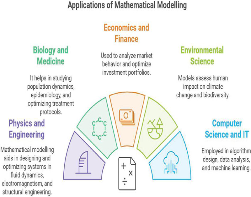
Figure 4 These are several applications of mathematical modelling.

3 Conclusion

Mathematical modelling is crucial across several domains and disciplines, offering a systematic and statistical structure for evaluating and understanding complex methods. It allows researchers, scientists, and engineers to simulate, forecast, and optimize diverse systems and processes which results in superior decision-making, improved designs, and successful resource allocation. Mathematical models allow the examination of various situations like the identification of basic patterns and connections, and the formation of ideas to continue research. They serve as effective tools for generating accurate predictions assessing conceptual ideas, and making policy decisions. Also, mathematical modelling promotes multidisciplinary work by connecting conceptual structures with experimental practices and promoting creativity across several fields. Mathematical modelling provides numerous benefits, such as reducing intricate events, enhancing decision-making, validating theories, optimizing systems, and promoting interdisciplinary collaboration. Mathematical models serve as fundamental tools for understanding, planning, and improving our environment. Through the use of mathematical concepts, tools, and algorithms, researchers can acquire deep understanding into the behaviour of complex systems that promote progress in science, technology, and society across all sectors.

References

[1] Blomhøj, M. (2004). Mathematical modelling: A theory for practice. In International perspectives on learning and teaching mathematics (pp. 145–159). National Center for Mathematics Education.

[2] Blomhøj, M., and Kjeldsen, T. H. (2006). Teaching mathematical modelling through project work: Experiences from an in-service course for upper secondary teachers. ZDM, 38(2), 163–177.

[3] Berry, J., and Houston, K. (1995). Mathematical modelling. Gulf Professional Publishing.

[4] Lahrouz, A., Omari, L., Kiouach, D., and Belmaâti, A. (2011). Deterministic and stochastic stability of a mathematical model of smoking. Statistics & Probability Letters, 81(8), 1276–1284.

[5] Kumar, A., Goel, K., and Nilam. (2020). A deterministic time-delayed SIR epidemic model: mathematical modelling and analysis. Theory in biosciences, 139(1), 67–76.

[6] Steinhoff, J., and Underhill, D. (1994). Modification of the Euler equations for “vorticity confinement”: Application to the computation of interacting vortex rings. Physics of Fluids, 6(8), 2738–2744.

[7] Aguirregabiria, V., and Magesan, A. (2013). Euler equations for the estimation of dynamic discrete choice structural models. In Structural Econometric Models (Vol. 31, pp. 3–44). Emerald Group Publishing Limited.

[8] Mesbah, A. (2016). Stochastic model predictive control: An overview and perspectives for future research. IEEE Control Systems Magazine, 36(6), 30–44.

[9] Valor, A., Caleyo, F., Alfonso, L., Velázquez, J. C., and Hallen, J. M. (2013). Markov chain models for the stochastic modelling of pitting corrosion. Mathematical Problems in Engineering, 2013(1), 108386.

[10] Berthiaux, H., and Mizonov, V. (2004). Applications of Markov chains in particulate process engineering: a review. The Canadian journal of chemical engineering, 82(6), 1143–1168.

[11] Mallet, J. L. (1997). Discrete modelling for natural objects. Mathematical geology, 29, 199–219.

[12] Szabó, B., and Babuška, I. (2021). Finite element analysis: Method, verification and validation.

[13] Krumsiek, J., Pölsterl, S., Wittmann, D. M., and Theis, F. J. (2010). Odefy-from discrete to continuous models. BMC bioinformatics, 11, 1–10.

[14] Ansorge, R., and Sonar, T. (2009). Mathematical models of fluid dynamics: modelling, theory, basic numerical facts-An introduction. John Wiley & Sons.

[15] Norton, T., Sun, D. W., Grant, J., Fallon, R., and Dodd, V. (2007). Applications of computational fluid dynamics (CFD) in the modelling and design of ventilation systems in the agricultural industry: A review. Bioresource technology, 98(12), 2386–2414.

[16] Macal, C. M., and North, M. J. (2009, December). Agent-based modelling and simulation. In Proceedings of the 2009 winter simulation conference (WSC) (pp. 86–98). IEEE.

[17] Scott, G., and Richardson, P. (1997). The application of computational fluid dynamics in the food industry. Trends in Food Science & Technology, 8(4), 119–124.

[18] Caunhye, A. M., Nie, X., and Pokharel, S. (2012). Optimization models in emergency logistics: A literature review. Socio-economic planning sciences, 46(1), 4–13.

[19] Sawik, B. (2023). Space mission risk, sustainability and supply chain: review, multi-objective optimization model and practical approach. Sustainability, 15(14), 11002.

[20] McCullagh, P. (2002). What is a statistical model?. The Annals of Statistics, 30(5), 1225–1310.

[21] van de Schoot, R., Depaoli, S., King, R., Kramer, B., Märtens, K., Tadesse, M. G., … and Yau, C. (2021). Bayesian statistics and modelling. Nature Reviews Methods Primers, 1(1), 1.

[22] English, L. D., and Halford, G. S. (2012). Mathematics education: Models and processes. Routledge.

[23] Lindell, D. B., Martel, J. N., and Wetzstein, G. (2021). Autoint: Automatic integration for fast neural volume rendering. In Proceedings of the IEEE/CVF Conference on Computer Vision and Pattern Recognition (pp. 14556–14565).

[24] Fornberg, B. (2021). Improving the accuracy of the trapezoidal rule. SIAM Review, 63(1), 167–180.

[25] Venkateshan, S. P., and Swaminathan, P. (2023). Numerical integration. In Computational Methods in Engineering (pp. 353–440). Cham: Springer International Publishing.

[26] Kaiser, G. (2020). Mathematical modelling and applications in education. Encyclopedia of mathematics education, 553–561.

[27] Mayovets, Y., Vdovenko, N., Shevchuk, H., Zos-Kior, M., and Hnatenko, I. (2021). Simulation modelling of the financial risk of bankruptcy of agricultural enterprises in the context of COVID-19. Journal of Hygienic Engineering and Design. 2021. Vol. 36. P. 192–198.

[28] Kaczor, Z., Buliński, Z., and Werle, S. (2020). modelling approaches to waste biomass pyrolysis: a review. Renewable Energy, 159, 427–443.

Biographies

Simran Sahlot is a Ph.D. scholar in Mathematics at Lovely Professional University, Punjab, under the supervision of Dr. Geeta Arora. Her research focuses on developing advanced numerical methods and mathematical models to solve real-world problems with applications in engineering and the sciences. She has presented her work at national and international conferences.

Geeta Arora earned her Ph.D. from IIT Roorkee, India, in 2011 and is a Professor in the Department of Mathematics at Lovely Professional University, Punjab. With over 12 years of teaching experience, she has published around 55 Scopus-indexed research papers, authored 15 book chapters, and written books on Vedic Mathematics and Essential Statistics. She has also edited and contributed to books with publishers like Taylor & Francis, IGI Global, and Elsevier. Her research focuses on developing numerical methods and statistics. A recipient of multiple research appreciation awards, she has supervised seven Ph.D. scholars and is currently guiding six more. Dr. Arora frequently conducts workshops on MATLAB and Vedic Mathematics, sharing her expertise with students and faculty.