Shortest Path of a Random Graph and its Application

Laxminarayan Sahoo^* and Rakhi Das

Department of Computer and Information Science, Raiganj University, Raiganj-733134, West Bengal, India
E-mail: lxsahoo@gmail.com; rakhidas2004@gmail.com
*Corresponding Author

Received 21 January 2024; Accepted 26 March 2024; Publication 13 April 2024

Abstract

The goal of this work is to provide an effective method for determining the shortest path in random graphs, which are complicated networks with random connectivity patterns. We have developed an algorithm that can identify the shortest path for both weighted and unweighted random graphs to accomplish our objective. As connectivity in these types of structures is changing, the algorithm adjusts to different edge weights and node configurations to provide fast and precise shortest path searching. The study shows that the suggested method performs more successfully in finding the shortest path throughout random graphs using comprehensive computations. Many networks, including social networks, granular networks, road traffic networks, etc., include nodes that can connect to one another and create random graphs in the present-day computational era. The outcomes demonstrate how flexible it is, which makes it a useful tool for practical uses in domains where random graph structures are common, like transportation networks, communication systems, and social networks. For illustration, we have taken into consideration an actual case study of communication road networks here. We have determined the shortest path of the road networks using our proposed algorithm, and the results have been presented. Better decision-making across a range of areas is made possible by this study, which advances effective algorithms designed for complicated and unpredictable network environments.

Keywords: Random graph, shortest path, probability distribution, weighted graph, unweighted graph.

1 Introduction

Over time, advancements in computation, optimization, and upgrading have led to an increased focus on optimal path selection for networks since the invention of the computer. There is a constant effort made by researchers to implement the best path selection algorithm. Graph theory now plays a significant part in the mathematical modeling of any network system. In 18th-century Swiss mathematician Leonhard Euler introduced the key concept of graph theory. The field of graph theory has been growing rapidly thereafter. There are currently numerous areas of investigation in graph theory [1]. The nomenclature of both nodes and edges is crucial for visually representing a network. Examining brain networks is a major topic of scientific inquiry, despite being represented by an undirected graph. Scientists and network researchers have established the theory that brain networks might be a mixed directional combination of directed and undirected [2]. Road networks are another example of this type of system; some have a direction from a source to a destination, while others have no direction at all. For notable contributions to the analyses of various graph-related topics, one might refer to the works of Thorup [3], Katerinis and Tsikopoulosk [4], Orlin et al. [5], Wang et al. [6], Jicy and Mathew [7], Li and Li [8], Bonato et al. [9], Mohammed [10], Sotskov [11], Deen et al. [12] etc. Additionally, several methods have been developed that use graph theory to find a complex network’s shortest path. The works of Triana and Syahputri [13], Sahoo et al. [14], Singh and Mishra [15], Brodnik et al. [16], Ramadiani et al. [17] and others might be consulted for additional information. Random graph (RG) is another term for a different kind of specialized graph that is used in the literature [18, 19]. The pioneering work of Paul Erdõs and Alfréd Rényi, who established the Erdõs-Rényi model [18] in the late 1950s, is the foundation of the study of random graphs. Based on this approach, graphs with different levels of connection are produced by assuming that edges between pairs of nodes have a probability distribution. Numerous random graph models, each capturing distinct features of real-world networks, have been developed by researchers since then. Hence, simply a probability distribution over graphs is commonly referred to as random graphs in mathematics. A basic model for analyzing the basic complexity and chaotic character of many real-world networks is a random graph. Random graphs serve as mathematical representations of a wide range of systems, including social networks, biological interactions, and communication infrastructures. As such, they offer an invaluable foundation for comprehending the emergent characteristics and activities of complex structures. Models of random graphs (RGs) are essential to complex network investigation. They support comprehension, management, and forecasting of events that take place, for example, in biological, social, and Internet networks. Basic bipartite networks, such as affiliation networks, and simple unipartite networks, such as acquaintance networks, are covered by the models [20]. Caimo and Friel [21] have examined Bayesian inference for estimating exponential random graph models (ERGMs), which are among the most significant models in several study fields like social network analysis, physics, and biology. Investigation has been done by Robins et al. [22] on recent advances in exponential random graph (p $^{*}$ ) models for social networks. In this study, they analyzed the work of Snijders et al. [23] and show how they fit empirical network data better than homogeneous Markov random graph models. Snijders conducted studies on Markov Chain Monte Carlo Estimation of Exponential Random Graph (ERG) Models [24]. The Robbins-Monro algorithm for estimating a solution to the likelihood equation serves as the foundation for the estimation procedures that are taken into consideration when simulating this ERG model using Gibbs or Metropolis Hastings sampling. Bollobás et al. [25] examined the diameter of a scale-free random graph. In this study, a random network process has been examined, in which vertices are linked to a fixed number m of earlier vertices, once at a time, and each earlier vertex is selected with a probability that is proportional to its degree. Aiello et al. [26] investigated a random graph model for power law graphs. A model for random graphs has been provided here, and it is essentially a particular instance of dense randomized graphs with degree sequences that obey a power law. Log size and log-log growth rate are two of the few parameters used in this approach. Nobari et al. performed studies on fast random graph generation [27]. In this study, an alternative data parallel approach for the Erdõs-Rényi model of random graph generation has been proposed and implemented it in a graphics processing unit (GPU). The weighted random graph (WRG) model has been introduced by Garlaschelli [28]. It is the weighted analogue of the Erdos–Renyi random graph and offers basic understanding of complex weighted networks. Garlaschelli also showed analytically that the geometric weight distribution, binomial degree distribution, and negative binomial strength distribution are basic features of the WRG. Janson et al. [29] explored bootstrap percolation on the random graph $G n, p$ . The idea of average distance in a random graph with predetermined predicted degrees has been studied by Chung and Lu [30]. Random graphs with clustering have been suggested by Newman et al. [31]. A network that exhibits transitivity, or the propensity for two neighbours of a network node to also be neighbours of one another, or clustering, has a long-standing challenge in network theory that has been resolved in this study. It is important to mention that filtering random graphs plays a crucial role in signal processing. Isufi et al. [32] have proposed filtering random graph processes over random time-varying graphs. Space-time signal-to-interference-and-noise-ratio (SINR) random graph optimum pathways have been examined by Baccelli et al. [33]. When modeling packet transmissions in wireless networks, these random graphs appear. A study on shortest paths in graphs with random weights has been conducted by Hassin and Zemel [34]. The shortest pathways between every pair of nodes in a directed or undirected complete graph with uniformly and independently distributed edge lengths in [0, 1] have been taken into consideration. To identify the shortest paths between given source/destination pairs while avoiding path overlaps at nodes, De Bacco et al. [35] addressed shortest node-disjoint paths on random graphs. A random graph is used to model how a molecular network forms from multifunctional antecedents. A random graph approach to multifunctional molecular networks has been suggested by Kryven et al. [36]. Floating time is particularly important since all routers in a subnet or autonomous domain must have the same, consistent picture of the network architecture to provide high quality multimedia services like file transfers, real-time video, telephone, etc. over an Internet like future network. Van Der Hofstad et al. have suggested the flooding time in random graphs [37]. For wireless actuator networks, Onat and Stojmenovic [38] examined the generation of random graphs. It presents a preliminary investigation into the generation of connected actuator graphs (CAG) using fast methods and what type of desirable properties can be obtained in comparison with entirely random networks, particularly for sparse node densities. Constrained random walks on random graphs are suggested by Servetto and Barrenechea [39] as routing algorithms for massive wireless sensor networks. Yang et al. [40] conducted studies on link prediction in brain networks based on a hierarchical random graph model. Link predict ion employs information about the brain network, including node properties and observable links, to estimate the probability that links exist between nodes. This study, which is based on a hierarchical random graph model with maximum likelihood estimation, plays a significant role in addressing the issue of the ineffectiveness of general link prediction methods applied to brain networks. Klootwijk et al. [41] have looked at the probabilistic analysis of optimization problems on generalized random shortest path metrics. The primary goal of this research is to generalize Erdős–Rényi random graphs. By providing separate random edge weights to each edge in the graph and determining the length of a shortest path between each pair of vertices with respect to the weights, one can develop a random shortest path metric. Kivimäki et al. [42] have investigated advancements in the theory of randomized shortest paths with a comparison of graph node lengths. This paper extends the theory of a particular family of graph node distances, based on statistical physics, called the randomized shortest path dissimilarity. The significance of random graphs presented in this introduction, with a focus on how they may be used to describe complex connection patterns and make it easier to analyze phenomena in which irregularity is important. Most of the published works that have been presented here have nothing to do with determining the shortest path for either directed or undirected random graphs. Thus, we have attempted to put into practice an algorithm that determines the shortest path of random graphs. Using our suggested algorithm, we have found the shortest path of the road networks, which are represented in terms of random graphs, and the results have been displayed in this paper. For the sake of illustration, an actual case study has also been solved and the outcomes have been provided.

2 Definition and Preliminaries

To develop the paper, we have provided a few definitions and explanations. In this section, we have defined a few key terms related to our suggested work and explained what they mean by way of notations. Notations and their meaning have been displayed in Table 1.

Table 1 Notation and their meaning

Notation	Meaning
$G = (V, E)$	It is the Graph with $V$ number of vertices and $E$ number of edges
$(u, v)$	An edge between two vertices
$G (N, L)$	It is a graph with $N$ nodes and $L$ links
$G (N, p)$	It is a graph with $N$ nodes with probability $p$ of connecting a pair of vertices
$d = (V, W)$	Denoted the distance
$X \sim N (μ, σ^{2})$	$X$ is a random variable which follow normal distribution with mean $μ$ and standard deviation $σ$

Definition 2.1 (Random Graph) In mathematics a random graph is a generic term for probability distributions over graphs. The theory of random graphs lies in the boundary between graph theory and probability theory. So, in general a graph $G = (V, E)$ is a random graph in which an edge $(u, v)$ appears with certain probability values $p$ .

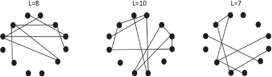
Figure 1 Random Graph of $G (N, L)$ Model with $N = 12$ and $p = \frac{1}{6}$ .

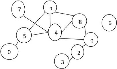
Figure 2 Random graph for $G (N, p)$ model.

2.1 Type of Random Networks/Graphs

In the random graph theory, generally, there are two types of random graphs viz. $G (N, L)$ Model and $G (N, p)$ Model (see Figures 1 and 2). These two models are as follows:

(i) $G (N, L)$ Model: $N$ labeled nodes are randomly connected to the $L$ Placed Link.

(ii) $G (N, p)$ Model: $N$ nodes with probability $p$ of connecting a pair of vertices $L$ number of links from a random network generated according to the $G (N, p)$ model.

Table 2 Some other type probability distributions

Distribution	Description	Example
Binomial	Describes variables with two possible outcomes. It is the probability distribution of the number of successes in $n$ trials with $p$ probability of success.	The number of times a coin lands on heads when you toss it five times
Discrete uniform	Describes events that have equal probabilities.	The suit of a randomly drawn playing card
Poisson	Describes count data. It gives the probability of an event happening k number of times within a given interval of time or space.	The number of text messages received per day

Definition 2.2 (Shortest path) A well-known idea in graph theory is the Shortest Path Algorithm. A path with the smallest distance between two vertices (or nodes) is found using the shortest path algorithm.

Shortest path of weighted Graph If the Graph is weighted, it is a path with the minimum sum of edge weights. The distance from the source vertex to the destination vertex is denoted by $d = (V, W)$ where the path’s weight is represented by $V$ and $W$ .

Shortest path of unweighted Graph In case of unweighted graphs, there will be no edge weights. In that case, the shortest path $P$ will become between the given two vertices with the minimum number of edges. Let $G = (V, E)$ be an undirected graph with $E$ edges and $V$ vertices. Let $P$ be the shortest path between any two vertices in the Graph such that there is no other path between any two vertices whose sum of edge weights is less than the sum of edge weights.

Definition 2.3 (Probability distribution) A probability distribution is the mathematical function that provides a chance of occurring for many possible experiment outcomes in probability theory and statistics. Probability distributions are often represented using graphs or probability tables. For example, $X \sim N (μ, σ^{2})$ ; $X$ is a random variable which follow normal distribution with mean $μ$ and standard deviation $σ$ . Table 2 contains a list of some other type probability distributions.

3 Algorithm for Random Graph’s Shortest Path

We have presented an algorithm in this section to find a random graph’s shortest path. There is no effort to determine the shortest path of a random graph, either for weighted or unweighted, in the literature that is available now. We developed algorithms that work with weighted and unweighted random graphs for this reason.

3.1 Algorithm for Shortest Path of a Weighted Random Graph

Here, we have provided the Algorithm for identifying the shortest path of a weighted random graph.

Input: Create a set of all unvisited sets ( $G_{r}, v, d, l$ )

Output: Evaluate the shortest path of a random graph.

Step 1: Initialize the vertices $(v_{0} - v_{n})$

Step 2: Choose two random vertices $v_{i}$ and $v_{j}$ .

Step 3: Follow the following steps for $(v_{n} - 1)$ vertices

Initially $d_{i j} = α [d_{i j} = distance between v_{i}, v_{j}]$

Now, finding the maximum probability distribution $p$ to connect the link between $v_{i}, v_{j}$

for $i = 0$ to $i < l_{n}$

if $(P_{N} (d_{i j}) > l_{n})$ $[l_{n} = links between v_{i}, v_{j}]$

then connect link between the vertices $v_{i}, v_{j}$ .

Create a random graph with at most $(v * (v - 1) / 2)$ links.

Step 4: Now follow the following steps of the random Graph $G_{r} = (v, e)$ for $(v - 1)$ vertices

Assign the initial vertices of the random Graph

dist $[v_{s}] = 0$

and

dist $[v_{n}] = α$ [For all unvisited node $v_{0}, v_{1}, \dots, v_{n}]$ .

Update all adjacent vertices

if $d (u) + l (u, v) < d (u)$

then $d (v) = d (u) + l (u, v)$

Step 5: Repeated the steps until all vertices are not updated $((| v |) - 1)$ (if there are $(| v |)$ vertices).

Step 6: Evaluate the shortest path of the random Graph.

3.2 Pseudo Code for Evaluating the Shortest Path of a Weighted Random Graph

Algorithm shortest path $S R (G_{r}, v, d, l)$

Initialize the vertices $(v_{0} - v_{n})$

Choose two random vertices $v_{i}$ and $v_{j}$

Initially $d_{i j} = α [d_{i j} = distance between v_{i}, v_{j}]$

for $i = 0$ to $i < l_{n}$

if $(P_{N} (d_{i j}) > l_{n})$ $[l_{n} = links between v_{i}, v_{j}]$

then connect link between the vertices $v_{i}, v_{j}$

Print (“A random graph is generated”)

$G_{r} = (v, e)$

dist $[v_{s}] = 0$

and

if $d (u) + l (u, v) < d (u)$

then $d (v) = d (u) + l (u, v)$

Return dist

Exit

The time complexity of the algorithm is $O (E \log V)$ .

3.3 Implementation of the Algorithm 7.3.2

The following steps are the implementation of our proposed algorithm for finding the optimal path of the random graph (see Figure 5). For this purpose, we have used Table 3 that provides details of probability distribution.

Table 3 Probability distribution table for connecting nodes

Random Set of Nodes	Distances of Nodes	Probability $p = \frac{1}{5}$ for Connecting the Nodes
$1 - 2$	20 km	0.2
$1 - 3$	6 km	0.2
$1 - 5$	7 km	0.2
1-4	3 km	0.2
3-2	9 km	0.2
4-2	4 km	0.2
5-2	8 km	0.2

Step 1: Initialize the set of vertices ${1, 2, 3, 4, 5}$ .

Step 2: Randomly choose two vertices are $1 - 2$ (see Figure 3) and the probability of distribution for connecting two vertices is $p = \frac{1}{5}$ , because in this network (see Figure 4) there are 5 nodes and there is a chance to connects two nodes is 1 because two nodes always only one edge in between them. And the dotted line shows the connection between the nodes and the solid line shows the shortest path of the network.

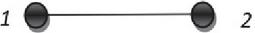
Figure 3 Randomly chosen two vertices namely 1 and 2.

Step 3: Random Graph is created based on the proposed algorithm mentioned in 3.1.

Figure 4 Random graph.

Step 4: Applying our proposed algorithm, we get the random Graph (see Figure 4) and the shortest path using the proposed algorithm is $(1 - 4 - 2)$ .

3.4 Algorithm for Shortest Path of an Unweighted Random Graph

Here, we have provided the Algorithm for identifying the shortest path of an unweighted random graph.

Step 1: Initialize the vertices $(v_{0} - v_{n})$ .

Step 2: Choose two random vertices $v_{i}$ and $v_{j}$ .

Step 3: Follow the following steps (4-10) for $(v_{n} - 1)$ vertices

Step 4: Initialize $dist [v] = {α}$

Step 5: $dist [s] = 0$

Step 6: $visited [v] = {f}$

Step 7: create a queue $q$ ; $q . push (s)$ and visited $[s] = t$

Step 8: $q \neq empty$

Step 9: $u = q . pop ()$

Step 10: continue for $(v - 1)$

$dist [v] = dist [u] + 1$

$visited [v] = t$

$q . push (v)$

Step 11: Exit

3.5 Pseudo Code for Evaluating the Shortest Path of an Unweighted Random Graph

Algorithm shortest path $S R (G_{r}, v, d, l)$

Initialize the vertices $(v_{0} - v_{n})$ .

Choose two random vertices $v_{i}$ and $v_{j}$ .

Initially $d_{i j} = α [d_{i j} = distance between v_{i}, v_{j}]$

for $i = 0$ to $i < l_{n}$

if $(P_{N} (d_{i j}) > l_{n})$ $[l_{n} = links between v_{i}, v_{j}]$

then connect link between the vertices $v_{i}, v_{j}$

Print (“A random graph is generated”)

$d i s t [v] = {α}$

$dist [s] = 0$

$visited [v] = {f}$

$q . push (s)$ and visited $[s] = t$

$(q \neq empty)$

{

$u = q . p o p ()$

or(every adjacent $v$ of $u$ )

{

$f (v \neq visited)$

{

$dist [v] = dist [u] + 1$

$q . push (v)$

}

The time complexity of the proposed algorithm $O (V + E)$ .

3.6 Implementation of the Algorithm

Implementing the Algorithm 3.5 creates a random graph (see Figure 5). Here, we randomly chosen a set of vertices ${0, 1, 2, 3, 4, 5}$ . Using our suggested algorithm, we have obtained the random graphs mentioned in Figures 5(a) to 5(f). Figure 5(f) gives the shortest path of the random graph depicted in Figure 5. Here, we have represented the visited nodes and generated queue in a tabular form in every step of the algorithm (See Tables 4 to 8)

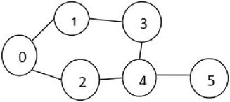
Figure 5 Random graph for model.

The step wise implementation of our proposed algorithm for unweighted random graphs is as follows:

Step 1: Initialize the set of vertices ${0, 1, 2, 3, 4, 5}$ .

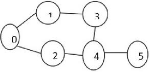
Figure 5(a): Unweighted random graph for model.

Step 2: In this step Table 4 is generated and the corresponding random graph is Figure 5(b).

Table 4 Visited node(s) and generated queue in step 2

Visited node	0
Queue	0

Figure 5(b): Random Graph with source node 0.

Step 3: In this step Table 5 is generated and the corresponding random graph is Figure 5(c).

Table 5 Visited node(s) and generated queue in step 3

Visited node	0	1	2
Queue	1	2

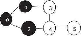
Figure 5(c): Shortest path of the random Graph is 0-1-2.

Step 4: In this step Table 6 is generated and the corresponding random graph is Figure 5(d).

Table 6 Visited node(s) and generated queue in step 4

Visited node	0	1	2	3
Queue	2	3

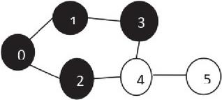
Figure 5(d): Shortest path of the random Graph is 0-1-2-3.

Step 5: In this step Table 7 is generated and the corresponding random graph is Figure 5(e).

Table 7 Visited node(s) and generated queue in step 5

Visited node	0	1	2	4
Queue	3	4

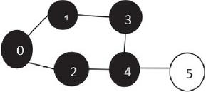
Figure 5(e): The shortest path of the random Graph is 0-1-2-3-4.

Step 6: In this step Table 8 is generated and the corresponding random graph is Figure 5(f).

Table 8 Visited node(s) and generated queue in step 6

Visited node	0	1	2	{4,0,1,2,3}	5
Queue	3	4

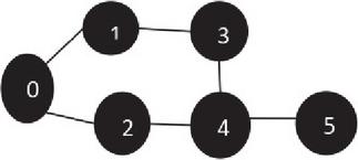
Figure 5(f): The shortest path of the random Graph is 0-1-2-3-4-5.

4 A Real Case Study (Survey Results)

We have considered a real case study to illustrate our proposed algorithm. Here, we have considered two districts namely Paschim Bardhaman and Birbhum of West Bengal, India, to describe the proposed study. To illustrate the study (mentioned in Section 3), we have connected two districts through a road network (see Figure 6) and the nodes of the road network are considered as places, and links between the nodes are considered as paths ( $P_{(i)}$ ) of two places. The nodes’ descriptions are mentioned in Table 9 and the distance of the nodes is mentioned in Table 10. Figures 6, 7 and 8 are Google maps of different nodes of the real case study in different scenario. Here, we have considered three scenarios viz. scenario-1, scenario-2 and scenario-3. The execution of the programming code of the proposed algorithm is successfully run in Python (version 3.6.15) editor. Hardware configurations of the computing machine are mentioned in Table 9.

Table 9 Details hardware configurations of computing machine

Processor	Intel(R) Core (TM) i3-7020U CPU @ 2.30GHz 2.30 GHz
Installed RAM	12.0 GB (10.4 GB usable)
System type	64-bit operating system, x64-based processor
Windows edition	10 Home Single Language
Version	21H2
Device’s name	Asus Vivobook15 Intel Core i3 7 $^{th}$ Gen

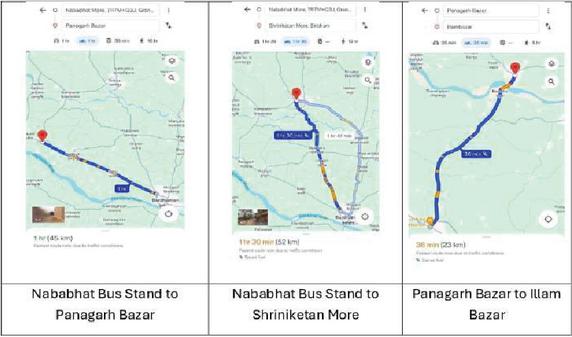
Figure 6 Google map of different nodes (Scenario-1).

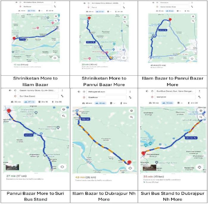
Figure 7 Google map of different nodes (Scenario-2).

Figure 8 Google map of different nodes (Scenario-3).

The Figure 9 is the graph representation with the help of Tables 10 and 11 mentioned here. Choose random nodes from Table 9 and for connecting the nodes we choose the probability $p = \frac{1}{8}$ , because in our network there are 8 nodes or places. Distance and probability distribution between Nodes are mentioned in Table 12. And there is chance to connect to node is 1 or two nodes are connected by only one link or edge.

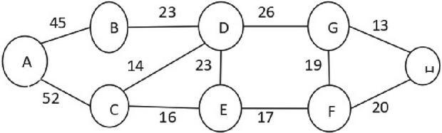
Figure 9 Representation of a road network in terms of graph.

4.1 Execution of Algorithm on Real Case Study

In this section we have generated random graph (see Figure 9(a)) and we have also generated graphs (see Figures 9(b) to 9(h)) in subsequent steps of the algorithm. Here, it is to be mentioned that doted lines represent the path which is optimal in a subsequent step of the proposed algorithm. Here, we have Initialized the set of vertices as ${A, B, C, D, E, F, G, H}$ and random graphs are created using the probability distribution mentioned in Table 12. Therefore, in this exaction process, we have considered probability value of each node as $p = 1 / 8 = 0.125$ (as every node has equally likely probable to connect the other nodes). Here, the input is the whole graph depicted in Figure 9(a). Using our proposed algorithm, we have executed the program in python language and we have obtained a series of outcomes obviously random graphs which are displayed in Figures 9(b) to 9(h). Finally, Figure 9(h) provides the shortest path. The path has been displayed using doted lines.

Table 10 Node description

Node	Place Name
A	Nababhat bus stand
B	Panagarh bazar
C	Shriniketan more
D	Illam bazar
E	Panrui bazar more
F	Suri bus stand
G	Dubrajpur Nh more
H	Bakreswar

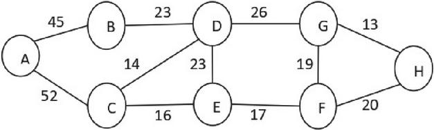
Figure 9(a): Random graph.

Table 11 Distance between nodes

Node	Place Name	Distance
$A - B$	Nababhat Bus Stand – Panagarh Bazar	45 km
$A - C$	Nababhat Bus Stand – Shriniketan More	52 km
$B - D$	Panagarh Bazar – Illam Bazar	23 km
$C - D$	Shriniketan More – Illam Bazar	14 km
$C - E$	Shriniketan More – Panrui Bazar More	16 km
$D - E$	Illam Bazar – Panrui Bazar More	23 km
$E - F$	Panrui Bazar More – Suri Bus Stand	17 km
$D - E$	Illam Bazar – Dubrajpur Nh More	26 km
$F - G$	Suri Bus Stand – Dubrajpur Nh More	19 km
$H - G$	Dubrajpur Nh More – Bakreswar	13 km
$F - H$	Suri Bus Stand – Bakreswar	20 km

Table 12 Distance and probability distribution between nodes

Node	Probability Distribution $p = \frac{1}{8}$	Distance
$A - B$	0.125	45 km
$A - C$	0.125	52 km
$B - D$	0.125	23 km
$C - D$	0.125	14 km
$C - E$	0.125	16 km
$D - E$	0.125	23 km
$E - F$	0.125	17 km
$D - E$	0.125	26 km
$F - G$	0.125	19 km
$H - G$	0.125	13 km
$F - H$	0.125	20 km

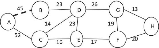
Figure 9(b): P $_{(1)}$ $=$ A-B.

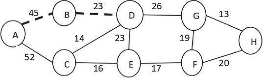
Figure 9(c): P $_{(2)}$ $=$ A-B-D.

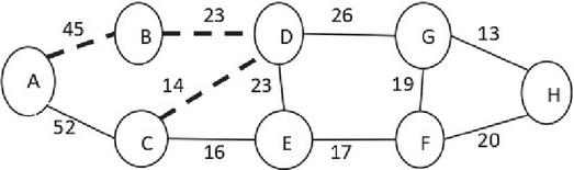
Figure 9(d): P $_{(3)}$ $=$ A-B-D-C.

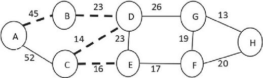
Figure 9(e): P $_{(4)}$ $=$ A-B-D-C-E.

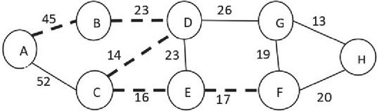
Figure 9(f): P $_{(5)}$ $=$ A-B-D-C-E-F.

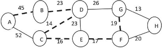
Figure 9(g): P $_{(6)}$ $=$ A-B-D-C-E-F-G.

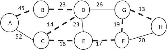
Figure 9(h): P $_{(7)}$ $=$ A-B-D-C-E-F-G.

The Shortest path of a random graph (see Figure 9) is P $_{s}$ $=$ P $_{(7)}$ $=$ A-B-D-C-E-F-G-H [where P $_{s}$ $=$ Shortest path].

5 Conclusion

The proposed study is help to evaluate the shortest path of weighted and unweighted random Graphs both. To evaluate the proposed algorithm, we can take the nodes randomly and then implanted a network according a predefine probability distribution. This study is very beneficiary for the social media, road transportation etc. to evaluate the shortest distances between the nodes. In future application of this study is finding shortest path of social media because previously it is impossible to calculate the shortest distance between the nodes or group of nodes in social media but our proposed algorithm able to evaluate the shortest distances between the nodes or of group of a social media. Because this study able to evaluate the shortest path of an unweighted graph. This study also has practical implementation for weighted graph. It gives a big impact for road transportation network because some time it is found that two nodes have no feasible connection but it has probability to connect a link. So, this study helps to finding the shortest path when this situation previously is not possible. In future we try to reduce the time complexity of our propose algorithm.

References

[1] Samanta, S., Pal, M., Mahapatra, R., Das, K., and Bhadoria, R. S. (2021). A study on semi-directed graphs for social media networks. International Journal of Computational Intelligence Systems, 14(1), 1034–1041.

[2] Sporns, O. (2018). Graph theory methods: applications in brain networks. Dialogues in clinical neuroscience, 20(2), 111–121.

[3] Thorup, M. (1997, October). Undirected single source shortest paths in linear time. In Proceedings 38th Annual Symposium on Foundations of Computer Science (pp. 12–21). IEEE.

[4] Katerinis, P., and Tsikopoulos, N. (2005). Edge-connectivity and the orientation of a graph. SUT Journal of Mathematics, 41(1), 1–10.

[5] Orlin, J. B., Madduri, K., Subramani, K., and Williamson, M. (2010). A faster algorithm for the single source shortest path problem with few distinct positive lengths. Journal of Discrete Algorithms, 8(2), 189–198.

[6] Wang, Z, H., Shi, S, S., Yu, L, and C., Chen, W, Z., (2012). An efficient constrained shortest path algorithm for traffic navigation, In Advanced Materials Research, 356, 2880–2885.

[7] Jicy, N., and Mathew, S. (2014). Some new connectivity parameters for weighted graphs. Journal of Uncertainty in Mathematics Science, 2014, 1–9.

[8] Li, S., and Li, Y. (2019). Semi-dynamic shortest-path tree algorithms for directed graphs with arbitrary weights. arXiv preprint arXiv:1903. 01756.

[9] Bonato, A., Delić, D., and Wang, C. (2016). The Structure and Automorphisms of Semi-directed Graphs. Journal of Multiple-Valued Logic & Soft Computing, 27, 161–173.

[10] Mohammed, A, M., (2017). Mixed graph representation and mixed graph isomorphism. Journal of Science. 30 (1), 303–310.

[11] Sotskov, Y. N. (2020). Mixed graph colorings: A historical review. Mathematics, 8(3), 385.

[12] Deen, Zeen El., M. R., and Omar, N. A. (2021). Extending of edge even graceful labeling of graphs to strong r-edge even graceful labeling. Journal of Mathematics, 2021, 1–19.

[13] Sahoo, L., Sen, S., Tiwary, K, S., Samanta, S., and Senapati, T., (2022). Modified Floyd–Wars hall’s Algorithm for Maximum Connectivity in Wireless Sensor Networks under Uncertainty. Discrete Dynamics in Nature and Society 2022, 1–11.

[14] Singh, A., and Mishra, P. K., (2014). Performance Analysis of Floyd-Warshall Algorithm vs Rectangular Algorithm, International Journal of Computer Applications, 107(16), 23–27.

[15] Brodnik, A., Grgurovic, M., and Pozar, R. (2022). Modifications of the Floyd-Warshall algorithm with nearly quadratic expected-time. Ars Math. Contemp., 22(1), 1.

[16] Bukhori, D., and Dengen, N. (2018, April). Floyd-warshall algorithm to determine the shortest path based on android. In IOP Conference Series: Earth and Environmental Science (Vol. 144, No. 1, p. 012019). IOP Publishing.

[17] Erdős, P., and Rényi, A. (1959). On random graphs I. Publ. math. debrecen, 6(290–297), 18.

[18] Barabási, A. L., and Albert, R. (1999). Emergence of scaling in random networks. science, 286(5439), 509–512.

[19] Drobyshevskiy, M., and Turdakov, D. (2019). Random graph modeling: A survey of the concepts. ACM computing surveys (CSUR), 52(6), 1–36.

[20] Caimo, A., and Friel, N. (2011). Bayesian inference for exponential random graph models. Social networks, 33(1), 41–55.

[21] Robins, G., Pattison, P., Kalish, Y., and Lusher, D. (2007). An introduction to exponential random graph (p*) models for social networks. Social networks, 29(2), 173–191.

[22] Snijders, T. A., Pattison, P. E., Robins, G. L., and Handcock, M. S. (2006). New specifications for exponential random graph models. Sociological methodology, 36(1), 99–153.

[23] Snijders, T. A. (2002). Markov chain Monte Carlo estimation of exponential random graph models. Journal of Social Structure, 3(2), 1–40.

[24] Bollobás, B., and Riordan, O. (2004). The diameter of a scale-free random graph. Combinatorica, 24(1), 5–34.

[25] Aiello, W., Chung, F., and Lu, L. (2001). A random graph model for power law graphs. Experimental mathematics, 10(1), 53–66.

[26] Nobari, S., Lu, X., Karras, P., and Bressan, S. (2011, March). Fast random graph generation. In Proceedings of the 14th international conference on extending database technology (pp. 331–342).

[27] Garlaschelli, D. (2009). The weighted random graph model. New Journal of Physics, 11(7), 073005.

[28] Janson, S., Łuczak, T., Turova, T., and Vallier, T. (2012). Bootstrap percolation on the random graph G_n,p.

[29] Chung, F., and Lu, L. (2004). The average distance in a random graph with given expected degrees. Internet Mathematics, 1(1), 91–113.

[30] Newman, M. E. (2009). Random graphs with clustering. Physical review letters, 103(5), 058701.

[31] Isufi, E., Loukas, A., Simonetto, A., and Leus, G. (2017). Filtering random graph processes over random time-varying graphs. IEEE Transactions on Signal Processing, 65(16), 4406–4421.

[32] Baccelli, F., Błaszczyszyn, B., and Haji-Mirsadeghi, M. O. (2011). Optimal paths on the space-time SINR random graph. Advances in Applied Probability, 43(1), 131–150.

[33] Hassin, R., and Zemel, E. (1985). On shortest paths in graphs with random weights. Mathematics of Operations Research, 10(4), 557–564.

[34] Bacco, C., Franz, S., Saad, D., and Yeung, C. H. (2014). Shortest node-disjoint paths on random graphs. Journal of Statistical Mechanics: Theory and Experiment, 2014(7), P07009.

[35] Kryven, I., Duivenvoorden, J., Hermans, J., and Iedema, P. D. (2016). Random graph approach to multifunctional molecular networks. Macromolecular Theory and Simulations, 25(5), 449–465.

[36] Van Der Hofstad, R., Hooghiemstra, G., and Van Mieghem, P. (2002). The flooding time in random graphs. Extremes, 5(2), 111–129.

[37] Onat, F. A., and Stojmenovic, I. (2007, June). Generating random graphs for wireless actuator networks. In 2007 IEEE international symposium on a world of wireless, mobile and multimedia networks (pp. 1–12). IEEE.

[38] Onat, F. A., and Stojmenovic, I. (2007, June). Generating random graphs for wireless actuator networks. In 2007 IEEE international symposium on a world of wireless, mobile and multimedia networks (pp. 1–12). IEEE.

[39] Servetto, S. D., and Barrenechea, G. (2002, September). Constrained random walks on random graphs: Routing algorithms for large scale wireless sensor networks. In Proceedings of the 1st ACM international workshop on Wireless sensor networks and applications (pp. 12–21).

[40] Yang, Y., Guo, H., Tian, T., and Li, H. (2015). Link prediction in brain networks based on a hierarchical random graph model. Tsinghua Science and Technology, 20(3), 306–315.

[41] Klootwijk, S., Manthey, B., and Visser, S. K. (2021). Probabilistic analysis of optimization problems on generalized random shortest path metrics. Theoretical computer science, 866, 107–122.

[42] Kivimäki, I., Shimbo, M., and Saerens, M. (2014). Developments in the theory of randomized shortest paths with a comparison of graph node distances. Physica A: Statistical Mechanics and its Applications, 393, 600–616.

Biographies

Laxminarayan Sahoo is currently an Associate Professor of Computer and Information Science, Raiganj University, Raiganj, India. He obtained his MSc from Vidyasagar University, India and his PhD from The University of Burdwan, India. He has received MHRD fellowship from Govt. of India and received Prof. M.N. Gopalan Award for Best PhD thesis in Operations Research from Operational Research Society of India (ORSI). He is a reviewer of several international journals and Academic Editor of International Journal “Mathematical Problems in Engineering,” Hindawi Publication. He is also Associate Editor of “Journal of Graphic Era University” River Publication. His specializations include, Wireless Sensor Network, Distributed Computing, Reliability Optimization, Genetic Algorithms, Particle Swarm Optimization, Graph Theory, Fuzzy Game Theory, Interval Mathematics, Soft Computing, Fuzzy Decision making and Operations Research. He has published a good number of articles in international and national journals of repute. Dr. Sahoo is the author of the books “Advanced Operations Research” published by Asian Books, New Delhi, “Advanced Optimization and Operations Research” published by Springer Nature, Singapore. He edited a book entitled “Real Life Applications of Multiple Criteria Decision – Making Techniques in Fuzzy Domain” published by Springer Nature and wrote several chapters from reputed publishers like Springer, IGI Global, CRC Press, Walter de Gruyter, McGraw-Hill and Elsevier. He is a fellow of ISROSET.

Rakhi Das received her B. Tech. from BIET Suri in 2006 & M. Tech. from NIT Durgapur in 2010. She is currently Pursuing Ph.D. in Computer and Information Science from Raiganj University since 2021. She has published two research paper in reputed international journal Mathematics published by MDPI and International Journal of Scientific Research in Mathematical and Statistical Sciences. Her main research work focuses on Graph Theory. She has 10 years of teaching experience.