Estimation and Assessment of Ionospheric Slant Total Electron Content (STEC) Using Dual-frequency NavIC Satellite System
Sharat Chandra Bhardwaj1,*, Anurag Vidyarthi1, B. S. Jassal1 and Ashish K. Shukla2
1Propagation Research Laboratory, Department of Electronics and Communication, Graphic Era (Deemed to be) University, Dehradun, India
2Space Applications Center, Indian Space Research Organization, Ahmedabad, India
E-mail: bhardwaj.sharat@gmail.com; dr.anuragvidyarthi@ieee.org; bsjassal@yahoo.co.in; ashish@sac.isro.gov.in
*Corresponding Author
Received 05 January 2021; Accepted 19 March 2021; Publication 29 June 2021
Abstract
Many atmospheric errors affect the positional accuracy of a satellite-based navigation device, such as troposphere, ionosphere, multipath, and so on, but the ionosphere is the most significant contributor to positional error. Since the ionosphere’s dynamics are highly complex, especially in low latitude and equatorial regions, a dual-frequency approach for calculating slant total electron content (STEC) for ionospheric delay estimation performs better in these conditions. However, the STEC is ambiguous and it cannot be used directly for ionospheric delay prediction, accurate positioning purposes, or ionospheric study. As a result, STEC estimation and pre-processing are required steps prior to any positioning application. There is very little literature available for STEC pre-processing in the NavIC system, necessitating an in-depth discussion. This paper focuses on how to extract navigational data from a raw binary file obtained from the Indian NavIC satellites, estimate and pre-process STEC, and build a database for STEC. It has been found that an hourly averaged STEC data is suitable for ionospheric studies and monthly mean value can be used for ionospheric behavioral research. Furthermore, the STEC is affected by diurnal solar activity, thus, the seven-month data analysis that includes summer and winter months has been used to study ionosphere action during the summer and winter months. It has been observed that STEC values are higher during the summer months than the winter months; some seasonal characteristics are also been found.
Keywords: Code range, Carrier range, NavIC, STEC, data pre-processing, Ionospheric delay.
1 Introduction
Satellite navigation systems are doing wonders in public as well as military applications. Earlier U.S.-based GPS was being used for Global Navigation Satellite Systems (GNSS) to provide coverage all over the world (COSTER et al., 1992). At present time other satellite systems such as GLONASS (Soviet Union), Galileo (European Union), BeiDou (China), QZSS (Japan) have been developed to provide global as well as regional coverage (Suryanarayana Rao, 2007). Recently, India has launched the seven satellite constellation of Indian Regional Navigation Satellite (IRNSS), with operational name NavIC (Navigation with Indian Constellation) to provide precision positioning over India and surrounded landmass (IRNSS SIGNAL-IN-SPACE ICD, 2017). In the NavIC seven satellite constellation three are in geostationary orbit at 32.5E, 83E, and 131.5E and four (two in each plane) are in inclined geosynchronous orbit (29) having their crossing longitudes 55E and 111.75E. The NavIC positioning services are transmitted on L5 (1165.45–1188.45 MHz) and S (2483.5–2500 MHz) band with central frequencies 1176.45 MHz and 2492.028 MHz (S1) respectively.
The positional accuracy of a satellite-based navigation system is influenced by many atmospheric errors such as troposphere, ionosphere, multipath, etc. but the major contributor in the positional error is the ionosphere (Mannucci et al., 1998). The received navigational signal experiences delay due to the presence of free electrons in the ionosphere which causes degradation of positional accuracy. To obtain this ionospheric delay, it is necessary to estimate the Slant Total Electron Content (STEC) between satellite and receiver.
To estimate and correct the delay present in satellite signal at the receiver, many ionospheric models have been proposed and are still widely being used for position correction. The single-frequency coefficient-based model is introduced by John A. Klobuchar for ionospheric time delay correction (Klobuchar, 1987). In this model, the ionospheric vertical delay is estimated by an amplitude and period varying cosine function depending upon the location of the receiver. The GPS broadcasts eight coefficients in the navigational signal which is used to determine the delay by forming a third-order polynomial. A constant value of 5 ns has been taken as a delay for the nighttime duration. Thus, with a known satellite geometry parameters (i.e. azimuth and elevation) the user can reduce the ionospheric range error up to 50%. The single-frequency systems are still widely being used for positioning and remote sensing radars for the estimation of ionospheric effect on the positioning. To determine the ionospheric time delay and thus error in range measurement, many ionospheric models have been developed. The European satellite navigation system is employing (Zhong et al., 2016) model for ionospheric delay correction. However, the characteristics of the ionosphere are highly dynamic, especially in equatorial and low latitude regions, and sometimes undergo severe solar magnetic storms; in such conditions static ionospheric delay prediction models can introduce a large amount of positioning error (Ratnam et al., 2017). In these conditions, a dual-frequency method performs better in the estimation of ionospheric delay (Hernández-Pajares et al., 2011). In this method the code and carrier phase range measurement from the satellites, at dual-frequency, are compared to calculate STEC which is further used for delay estimation.
The estimation of STEC from code and carrier phase measurement is not straightforward. The STEC estimated from dual-frequency code ranges are ambiguous; it includes random fast variations in magnitude due to ionospheric scintillation and signals multipath (Hager et al., 1991). Thus the STEC cannot be directly used for ionospheric delay estimation and precise positioning applications (Jakowski et al., 2011; Bhardwaj et al., 2020). However, the STEC derived from carrier phase range measurement is comparatively much smooth but an additional ambiguity that is integer carrier cycle needed to be determined (Bradford W. Parkinson & James J. Spilker Jr., 2013). This process of integer carrier cycles requires additional data processing steps and thus makes the STEC estimation more complex (Sinha et al., 2018). Hence, the estimation and pre-processing of STEC are essential steps before any positioning application. For the NavIC system, very little literature on STEC pre-processing (Bhardwaj et al., 2018; Ma et al., 2019) has been found which creates a requirement for an in-depth discussion on it. Moreover, the characterization of ionospheric behavior is essential for precise positioning and TEC modeling applications.
This paper focuses on how to extract navigational data from a raw binary file obtained from NavIC satellites, estimate and pre-process STEC, and build a database of STEC. Furthermore, the seasonal database of STEC for seven months (that includes summer and winter months) has been created and used for ionospheric behavioral analysis.
In Section 2, the typical data obtained from the NavIC satellites and using these data, the behavior of satellite constellation has been discussed. The theoretical background of STEC estimation has been discussed in Section 3. The diurnal and seasonal behavior of STEC along with the effect of time duration selection in data integration have been covered under the results and analysis heading in Section 4.
Table 1 Satellite data and values at L5 frequency
| Satellite Data | Values | |||||
| TOWC (s) | 0 | 1 | 2 | 3 | 4 | 5 |
| PRN | 2.0000 | 2.0000 | 2.0000 | 2.0000 | 2.0000 | 2.0000 |
| C/N (dB-Hz) | 47.5096 | 47.9837 | 47.7505 | 48.0220 | 48.5758 | 49.1990 |
| Azimuth (deg) | 228.5730 | 228.5761 | 228.5791 | 228.5822 | 228.5852 | 228.5882 |
| Elevation(deg) | 51.0979 | 51.0993 | 51.1006 | 51.1020 | 51.1033 | 51.1046 |
| PR (m) | 37157120.4066 | 37157036.098 | 37156952.391 | 37156868.09 | 37156784.026 | 37156700.76 |
| DR (m) | 84.0187 | 83.9589 | 84.0217 | 83.9548 | 83.9697 | 83.8808 |
| Carrier Delay (cycles) | 145812580.264 | 145812249.58 | 145811920.76 | 145811590.58 | 145811260.82 | 145810934.52 |
| Satellite X Pos. (m) | 25032591.5284 | 25032794.79 | 25032998.003 | 25033201.167 | 25033404.281 | 25033607.345 |
| Satellite Y Pos. (m) | 33746181.8992 | 33745837.109 | 33745492.292 | 33745147.445 | 33744802.57 | 33744457.667 |
| Satellite Z Pos. (m) | 4434301.7187 | 4435759.8785 | 4437218.0149 | 4438676.1278 | 4440134.2172 | 4441592.2832 |
| Satellite X Velocity (m/s) | 203.2878 | 203.2383 | 203.1889 | 203.1394 | 203.0899 | 203.0404 |
| Satellite Y Velocity (m/s) | 344.7754 | 344.8039 | 344.8325 | 344.8610 | 344.8896 | 344.9181 |
| Satellite Z Velocity (m/s) | 1458.1711 | 1458.1477 | 1458.1243 | 1458.1007 | 1458.0773 | 1458.0538 |
2 Data Collection
The IGS (IRNSS/GPS/SBAS) receiver is installed at Graphic Era University, Dehradun (31.26N and 77.99E). The raw binary data of NavIC, GPS, and GAGAN satellites are logged at every second in UTC (Coordinated Universal Time) format. The NavIC satellites (PRN 2 to PRN 7) data are available at dual frequency L5 and S1, whereas, the data of GPS and GAGAN are available at L1 frequency only. The data from PRN 1 is not available due to satellite clock failure. From the raw binary files, the satellite data are extracted into Comma Separated Value (CSV) file format using extraction feature in receiver GUI. The sample data for one satellite PRN 2 is given in Table 1, whereas a single CSV file contained 3 hours of data of NavIC satellites at one frequency. The typical data consists of Time of week count (TOWC) signal strength (C/N), azimuth & elevation angle, satellite code range; also called pseudorange (PR), Doppler range (DR), carrier delay, satellite position, and velocity (in geodetic XYZ coordinate system), etc. These data files are imported in MatLab software environment combined to form a 24-hour data file at both L5 and S1 frequencies. The combined data is converted from UTC to IST (Indian Standard time) format to facilitate analysis in terms of localized sun position (time of the day). In this paper, code range, Azimuth, Elevation data have been used and pre-processed for ambiguities such as missing data, zero or very high values, etc. for STEC estimation. The variations of azimuth and elevation angle of NavIC satellites (PRN 2–7) during 24 hours have been plotted in Figure 1. From the figure it can be observed that the variation in azimuth and elevation angles for geostationary (GEO) satellites (PRN 3,6,7) are very small as compared to geosynchronous (GSO) satellites (PRN 2,4,5); the minimum and maximum values of azimuth and elevation angles are given in Table 2. All satellites, except PRN 3, are having an elevation angle below 50 most of the time. Such condition requires special attention because most of the mathematical model for satellite navigation prefers elevation greater than 50 and low elevation could introduce error in positioning. By using azimuth and elevation data a sky plot has been shown in Figure 2 which gives a clear picture of satellite position and movement with respect to receiver position (red dot) during a day. There is a slight change in GEO’s position, while, GSO’s make a figure of eight in the sky; the path of PRN 4 and 5 are overlapped.
Table 2 Satellite Azimuth and Elevation data (Min. and Max.) during 24 hours on Jun. 5, 2017
| PRN | 2 | 3 | 4 | 5 | 6 | 7 | |
| Elevation | Min. | 18.4213 | 50.9081 | 13.6250 | 13.9717 | 26.9515 | 21.8579 |
| (Deg.) | Max. | 68.7271 | 57.7203 | 58.3479 | 58.1495 | 32.2524 | 27.3123 |
| Azimuth | Min. | 200.5060 | 168.5470 | 83.5900 | 84.3242 | 239.5562 | 107.6498 |
| (Deg.) | Max. | 272.7398 | 171.2036 | 149.1695 | 148.9667 | 248.1551 | 115.7819 |
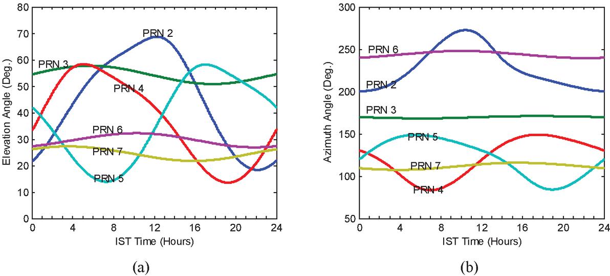
Figure 1 Diurnal (a) Elevation angle (b) Azimuth angle variation of Satellites PRN 2–7 on Jun. 5, 2017.
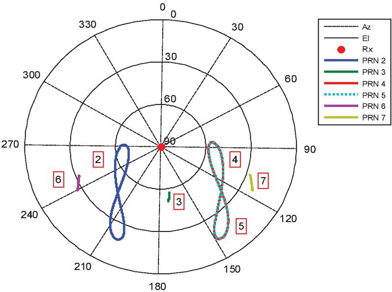
Figure 2 Diurnal Sky plot of NavIC satellites (PRN 2–7) on Jun. 5, 2017.
3 Determination of Slant Total Electron Content (STEC)
Corrections for ionospheric range rate errors for a single frequency user are not practical by ionospheric electron content modeling techniques due to the lack of predicting the uncertain and dynamic behavior of ionospheric phenomena, which produce range errors of a few seconds to minutes. Also, non-frequency dependents effects such as satellite clock offset, satellite orbital error, multipath, etc. are present in the measurement and needed to calculate for corrected code range. The most efficient method to eliminate the ionospheric and other range errors is by using measurements at dual-frequency signals.
In the dual-frequency method code range and/or carrier phase measurements at dual frequency are used to reconstruct the ionosphere Total Electron Content (TEC). This dual-frequency method is the main reason why the GNSS signal has two carrier waves. The STEC can be determined by taking the difference between code range and/or carrier phase measurements at dual frequencies. Furthermore, the STEC can be used for ionospheric range error calculation. The dual-frequency method also eliminates non-frequency dependent errors such as tropospheric delay, orbital errors, and clock errors.
A code range measurement is given by (Jin and Jin, 2011):
| (1) |
where, is the measured code range (in meters) at dual-frequency (i L5 and S1); R is the actual line of sight (LOS) range between satellite and receiver; is satellite orbital range error; is the speed of light; and are satellite and receiver clock offsets respectively; is ionospheric delay; is the tropospheric delay; is multipath delay; and is a delay due to receiver noise.
Using (1), the code range measurements at L5 and S1 can be expressed as
| (2) | |
| (3) | |
| (4) |
The ionospheric delay in (1) can be obtained as (Li and Jin, 2016):
| (5) |
where, is ionospheric plasma frequency, is carrier signal frequency, is a differential length, Ne is the density of electrons along LOS between satellite and receiver.
By neglecting the differential receiver noise term in (4) and from (5) it can be written as;
| (6) |
By putting the values of NavIC frequencies as f MHz and MHz in (6) the value of STEC can be written as (Bhardwaj et al., 2020)
| (7) |
where, .
4 Results and Analysis
The STEC has been calculated from code range and carrier phase measurements using Equation (7), at each epoch for PRN 2 to 7, and shown in Figure 3(a) for GSO and (b) GEO satellites separately for better analysis. In Figure 3(a), the GSO satellites have STEC peaks at different hours of the day while in the case of GEO satellites (Figure 3(b)) STEC peaks are during the same time duration (15 to 16 hrs.) This is because along with diurnal solar activity the STEC depends upon the elevation angle. For GSO satellites, with a decrease in elevation angle the path length between satellite and receiver increases and thus increase in STEC (as given in Equation (5)) values. In the case of GEOs, there are small variations in elevation angle as compared to GSOs and hence the STEC curves are mainly following the solar activity. Furthermore, as the code range measurements are ambiguous, a rapid fluctuation in STEC values can be observed in the curves. To remove these fast variations, a low-pass filter has been applied to STEC data and the resultant curves are shown in Figure 3(c) and (d) for GSOs and GEOs respectively. It can be observed from the figure that the fast fluctuations are greatly removed and slow changes in the STEC curves are now clearly visible. As the changes in ionospheric TEC are mainly due to diurnal solar activity, which is a gradual process, the abrupt variations in STEC curves are due to other ionospheric scintillation effects present in the code range measurement. Directly employing such STEC data for ionospheric studies and delay correction could lead to artificial changes in the observation. Thus a further data processing step that is data integration for a defined interval is required which can provide a mean value of data during that duration. Also, the STEC has been calculated at each epoch (logged at every second) leads to a large volume of data (86400 data points in 24 hours) and it will increase the data processing time and complexity in case of larger time duration analysis such as weekly, monthly and yearly. The integration of data based on time duration could solve these problems. The data integration steps, selection of optimal integration duration, and outcomes have been discussed below.
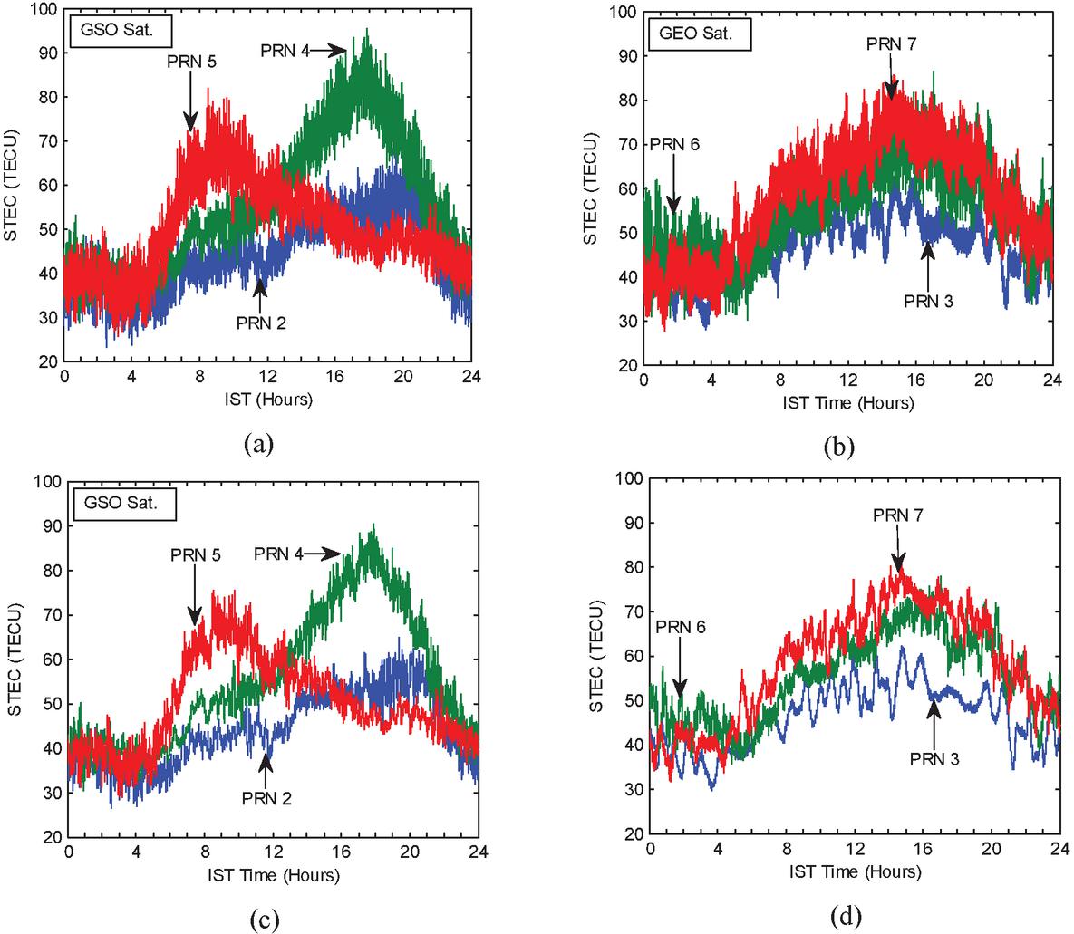
Figure 3 Estimated STEC from Code range for (a) GSOs (b) GEOs, and Filtered STEC for (c) GSOs (d) GEOs.
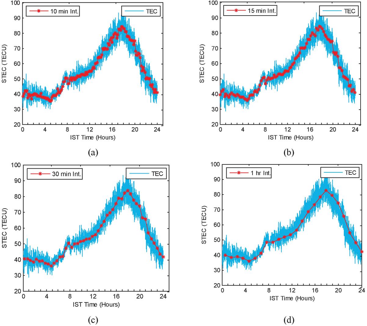
Figure 4 Diurnal variation of averaged TEC for different integration time for PRN 4 (a) 10 Min (b) 15 Min (c) 30 Min (d) 1 hour.
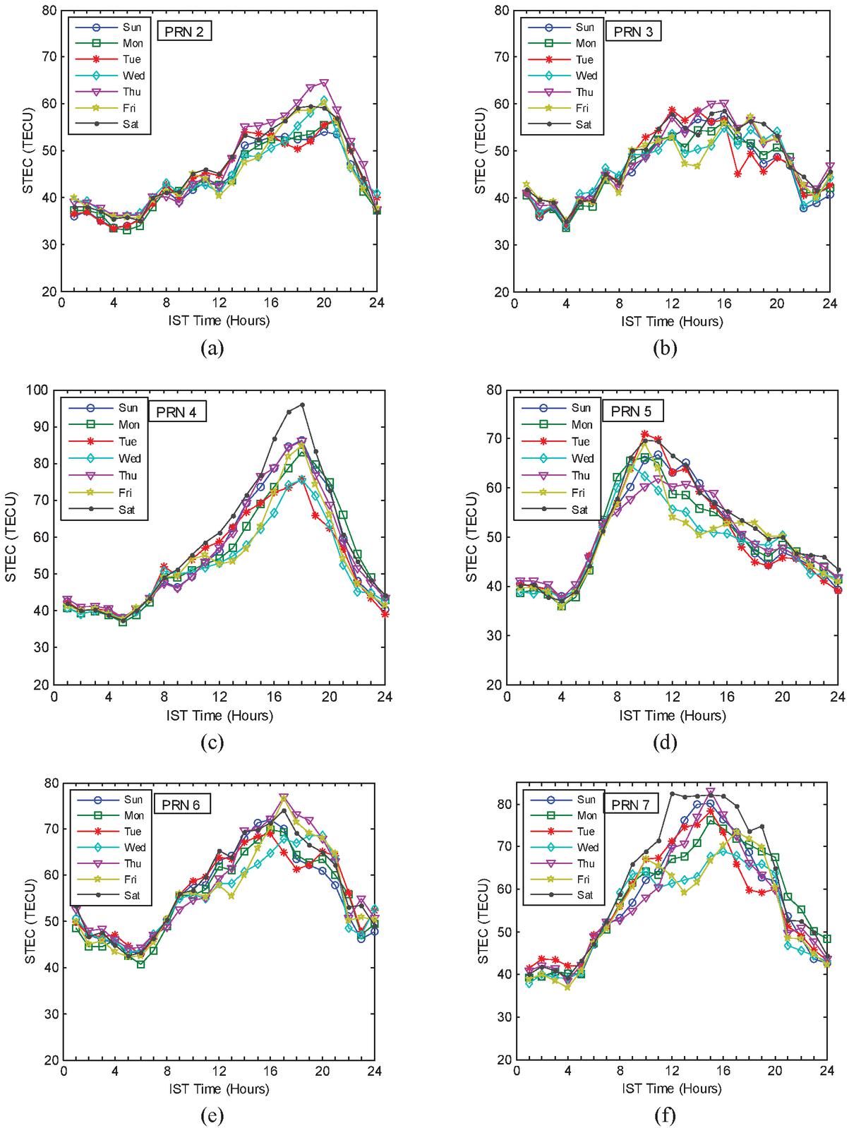
Figure 5 Diurnal STEC variation of (a) PRN 2, (b) PRN 3, (c) PRN 4, (d) PRN 5, (e) PRN 6, and (f) PRN 7, for one-week duration (04th to 10th June).
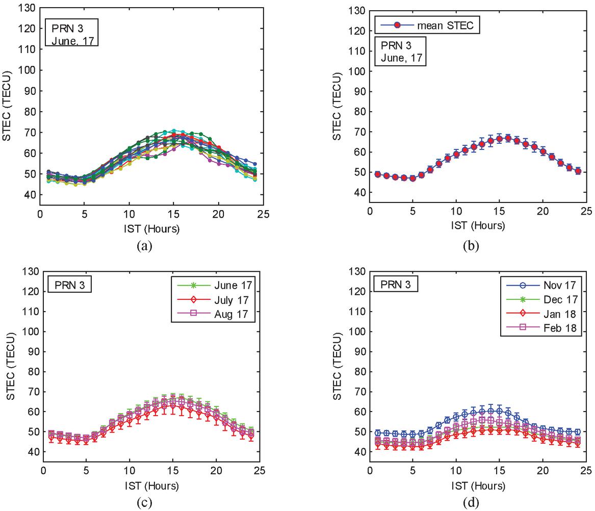
Figure 6 Diurnal STEC variation of PRN 3 (a) for June 2017 (b) monthly mean STEC (c) for summer months (d) for winter months.
In data integration, the most important step is the selection of integration time duration because the original behavior might get affected due to inappropriate time duration. If the integration time duration is very small it may inherit the fluctuations from the original curve, whereas a long duration might alter the shape of the curve. Diurnal variation of STEC is calculated for different integration times are shown in Figure 4 (a) 10 Min (b) 15 Min (c) 30 Min (d) 1 hour in which the integrated curves have been overlapped over the original curve. For 10, 15, and 30 min integration time duration (Figure 4 (a) (b) and (c)) it can be observed that the resultant curves consist of a sharp change in integrated data points. In the case of 1 hour integration time (Figure 4 (d)) the curve is much smoother as compared to other time durations and follows the mean behavior of the original curve. Another advantage of 1 hour integration time is that it drastically decreases the number of resultant data points, i.e. 24 only, in comparison to 144 for 10 min, 96 for 15 min, and 48 for 30 min duration. Thus 1-hour time duration has been selected for the data integration step for further analysis.
(a) Diurnal Analysis of STEC
For the analysis of diurnal variation of STEC, one week (From Sunday to Saturday) of data (04th to 10th June 2017) has been processed and plotted in figure for PRN 2 to 7. To study the characteristics of the ionosphere, plotted STEC curves can be divided mainly into four value zones i.e. minimum before sunrise (0–5 hrs), rise after sunrise and before afternoon (5–13 hrs), peak (13–16 hrs), and fall (16–18 hrs). In the minimum zone, the STEC curves for all satellites reach their minimum just before sunrise (i.e. 5 hrs) during the entire week as shown in Figure 5. This verifies the typical ion-recombination process in the ionosphere due to the absence of solar radiation. From Figure 5(a) to (f), it can be observed that the STEC curves experience a sharp rise after sunrise due to photo-electron generation in the ionosphere and continue to increase with solar radiations. The rising-rate, peak hours, and falling-rate of STEC of GEO satellites (Figure 5(c), (e), and (f)) are found similar, however, the GSO satellites (Figure 5(a), (c), and (d) are having different rising-rate, peak hours and falling-rate due to the combined effect of elevation angle and solar radiations as discussed previously. Another important characteristic, the presence of ionospheric disturbance can be identified from the STEC graph. The disturbance may be localized or cover the entire ionosphere, its duration could be a short time (minutes to hours) or last for the entire day. The unusual behavior of the STEC curve on Friday can be observed for all satellites, which indicate the presence of ionospheric disturbance during the entire day, whereas higher STEC peaks can be observed on Saturday for PRN 4 and 7 only, which shows the presence of localized disturbance. A similar analysis has been done for the monthly behavior of ionospheric TEC.
The STEC values were estimated for each hour of the day for seasonal analysis. The temporal variations of hourly average STEC values for June 2017 are plotted in Figure 6(a). From the figure, it can be observed that the curve patterns are almost identical except for a few days. The mean of these curves is thus plotted with standard deviation in Figure 6(b) for monthly analysis. The curves display almost similar activity (1 TEC) at morning (00:00 to 05:00hrs) and night (20:00 to 24:00), and are within 3 TECU) during the rest of the day. This shows the feasibility of taking the monthly mean of the STEC for further analysis.
(b) Seasonal Analysis of STEC
The monthly mean STEC curves for summer (i.e. June, July, and August), and winter (i.e. November, December, January, and February) months are grouped. The seasonal curves are plotted in Figure 6(c) and (d) for each satellite PRN 3 only for better understanding. From the figures, it can be observed that the STEC curves are having similar diurnal behavior i.e. minimum value, peak hours, but different seasonal characteristics, in terms of rising rate, peak values, and fall rate can be observed. The STEC values are higher during the summer months than the winter months. Although, in the summer and winter months STEC are having and similar diurnal variations, a higher nighttime value and slow falling rate can be observed during summer months that indicate the effect of ion temperature on electron density in the ionosphere.
5 Conclusion and Future Scope
In this paper, an in-depth discussion on the NavIC data logging, data extraction, satellite position and motion with respect to the receiver, and estimation and pre-processing of STEC have been done. It has been observed that NavIC satellites are having low elevation angles most of the time which requires special attention in any mathematical modeling because existing satellite navigation methods prefer elevation greater than 50 and low elevation could introduce error in positioning. The estimated STEC from code range measurement experiences fast fluctuation which has been reduced using a low pass filter. To eliminate unwanted slow variations in STEC and reduction in data volume a data integration step has been introduced and the 1-hour integration time duration has been found suitable for it. Using these steps a database of STEC has been prepared and plotted to analyze its diurnal variation for each PRN (2–7). It has been observed that the behavior of STEC for GEOs are similar and follows the diurnal solar variation, whereas, the STEC of GSOs is having different characteristics due to the combined effect of their elevations and solar radiation during the day. Furthermore, it has been found that the STEC curves can detect the ionospheric disturbance as well as its characteristics such as short-term, long-term, localized, and regional effects. A similar analysis has been done for the monthly and seasonal behavior of ionospheric TEC. The STEC curves are having similar diurnal behavior but different seasonal characteristics. The STEC are higher during the summer months than the winter months and a higher nighttime value and slow falling rate can be observed during summer months that indicate the effect of ion temperature on electron density in the ionosphere.
References
Bhardwaj, S. C., Vidyarthi, A., Jassal, B. S., and Shukla, A. K. (2020). Estimation of Temporal Variability of Differential Instrumental Biases of NavIC Satellites and Receiver using Kalman Filter. Radio Science. https://doi.org/10.1029/2019RS006886
Bhardwaj, S. C., Vidyarthi, A., Jassal, B. S., and Shukla, A. K. (2020). Investigation of ionospheric total electron content (tec) during summer months for ionosphere modeling in Indian region using dual-frequency NavIC system. Advances in Intelligent Systems and Computing, 1166, 83–91. https://doi.org/10.1007/978-981-15-5148-2_8
Bhardwaj, S. C., Vidyarthi, A., Jassal, B. S., and Shukla, A. K. (2018). Study of temporal variation of vertical TEC using NavIC data. 2017 International Conference on Emerging Trends in Computing and Communication Technologies, ICETCCT 2017, 2018-January, 1–5. https://doi.org/10.1109/ICETCCT.2017.8280317
Bradford W. Parkinson (Stanford University, Stanford, C. ), and James J. Spilker Jr. (Stanford Telecom, Sunnyvale, C. (2013). Global Positioning System: Theory and Applications (Vol. 53, Issue 9). https://doi.org/10.1017/CBO9781107415324.004
Coster, A. J., Gaposchkin, E. M., and Thornton, L. E. (1992). Real-Time Ionospheric Monitoring System Using GPS. Navigation, 39(2), 191–204. https://doi.org/10.1002/j.2161-4296.1992.tb01874.x
Hager, B. H., King, R. W., and Murray, M. H. (1991). System Global Positioning.
Hernández-Pajares, M., Juan, J. M., Sanz, J., Aragón-Àngel, À., García-Rigo, A., Salazar, D., and Escudero, M. (2011). The ionosphere: Effects, GPS modeling and the benefits for space geodetic techniques. Journal of Geodesy, 85(12), 887–907. https://doi.org/10.1007/s00190-011-0508-5
IRNSS Signal-in-Space ICD for SPS Version 1.0 Signal in Space ICD for Standard Positioning Service Configuration Definition Document Satellite Navigation Programme. (2017).
Jakowski, N., Mayer, C., Hoque, M. M., and Wilken, V. (2011). Total electron content models and their use in ionosphere monitoring. Radio Science, 46(5), 1–11. https://doi.org/10.1029/2010RS004620
Jin, S., and Jin, R. (2011). GPS Ionospheric Mapping and Tomography: A Case of Study in a Shanghai Astronomical Observatory, Chinese Academy of Sciences, Shanghai 200030, China Graduate University of the Chinese Academy of Sciences, Beijing 100049, China. 1127–1130. http://nssdcftp.gsfc.nasa.gov/models/ionospheric/iri/iri2007
Klobuchar, J. A. (1987). Ionospheric Time-Delay Algorithm for Single-Frequency GPS Users. IEEE Transactions on Aerospace and Electronic Systems, AES-23(3), 325–331. https://doi.org/10.1109/TAES.1987.310829
Li, J., and Jin, S. (2016). Second-order ionospheric effects on ionospheric electron density estimation from GPS Radio Occultation. International Geoscience and Remote Sensing Symposium (IGARSS), 2016-Novem, 3952–3955. https://doi.org/10.1109/IGARSS.2016.7730027
Ma, X., Tang, C., and Wang, X. (2019). The evaluation of IRNSS/NavIC system’s performance in its primary and secondary service areas–data quality, usability and single point positioning. Acta Geodaetica et Geophysica, 54(1), 55–70. https://doi.org/10.1007/s40328-019-00246-8
Mannucci, A. J., Wilson, B. D., Yuan, D. N., Ho, C. H., Lindqwister, U. J., and Runge, T. F. (1998). A global mapping technique for GPS-derived ionospheric total electron content measurements. Radio Science, 33(3), 565–582. https://doi.org/10.1029/97RS02707
Of Geophysics, A., and To, S. (2004). 8 Effects of gradients of the electron density on Earth-space communications (Vol. 47, Issue 3).
Ratnam, D. V., Dabbakuti, J. R. K. K., and Sunda, S. (2017). Modeling of Ionospheric Time Delays Based on a Multishell Spherical Harmonics Function Approach. IEEE Journal of Selected Topics in Applied Earth Observations and Remote Sensing, 10(12), 5784–5790. https://doi.org/10.1109/JSTARS.2017.2743695
Sinha, S., Mathur, R., Bharadwaj, S. C., Vidyarthi, A., Jassal, B. S., and Shukla, A. K. (2018, December 1). Estimation and smoothing of tec from navic dual frequency data. 2018 4th International Conference on Computing Communication and Automation, ICCCA 2018. https://doi.org/10.1109/CCAA.2018.8777665
Suryanarayana Rao, K. N. (2007). GAGAN – The Indian satellite based augmentation system. Indian Journal of Radio and Space Physics, 36(4).
Zhong, J., Lei, J., Dou, X., and Yue, X. (2016). Assessment of vertical TEC mapping functions for space-based GNSS observations. GPS Solutions, 20(3), 353–362. https://doi.org/10.1007/s10291-015-0444-6
Biographies

Sharat Chandra Bhardwaj is Ph.D. student at the Graphic Era (deemed to be University), Dehradun India. He received B.E. and M.Tech. degree in electronics and communication from Sant Longowal Institute of Engineering and Technology, Longowal, Punjab, India, in 2009 and 2011 respectively. He is currently a Research Fellow working with the Indian Space Research Organization, Ahmedabad, India. His area of interest includes signal propagation through the ionosphere.

Anurag Vidyarthi received B.Sc. degree from MJPR University, Bareilly, India, in 2005 and M.Sc. degree from BU Bhopal, India, in 2007. He receives M.Tech. and Ph.D. degree from Graphic Era University, India, in 2010 and 2014 respectively. Presently he is associated with Department of Electronics and Communication Engineering, Graphic Era University, Dehradun, India. His areas of interest are rain attenuation, fade mitigation techniques, ionospheric effects on the navigation system, and applications of Navigational satellite data.

B. S. Jassal received M.Sc. degree in Physics from Meerut University, Meerut, India, in 1968 and Ph.D. degree in Science (Radiowave propagation) from Jadavpur University, Calcutta, India, in 1990. He worked as lecturer in DAV (PG) College, Dehradun from July 1969 to October 1969. He worked in Defence Electronics Applications Laboratory (Defence Research & Development Organization, Govt. of India) as a scientist for 38 years from 1969 to 2007. He headed various research projects relating to RF and Microwave communication, Radiometric studies of the atmosphere, terminal guidance systems, satellite communication for military applications. Presently he is associated with Graphic Era University, Dehradun since 2008. In addition to teaching undergraduate and postgraduate students, he has also been involved in various sponsored research projects. His present area of research is NavIC system based ionospheric studies.

Ashish K. Shukla received the Masters and Ph.D. degrees in applied mathematics from Lucknow University, Lucknow, India, in 1997 and 2003 respectively. He is currently a scientist in the SATCOM and IT Application Area, with the Indian Space Research Organization (ISRO), India. His research interests include propagation modeling in the ionosphere and troposphere and NavIC applications.
Journal of Graphic Era University, Vol. 9_2, 137–156.
doi: 10.13052/jgeu0975-1416.923
© 2021 River Publishers