Constraints on Neutrino Mass Matrix with no Majorana Phases

Hiba Khan¹, Santosh Kumar Singh^1,* and Vivek Kumar Nautiyal²

¹Department of Applied Sciences and Humanities, Institute of Engineering and Technology, Lucknow 226021, India
²Department of Physics, Babasaheb Bhimrao Ambedkar University, Lucknow 226025, India
E-mail: 192000004@ietlucknow.ac.in; santoshsingh@ietlucknow.ac.in; viveknautiyal01@gmail.com
*Corresponding Author

Received 17 May 2022; Accepted 19 May 2022; Publication 22 July 2022

Abstract

In the basis where charged lepton mass matrix is real and diagonal, we have found conditions under which there are no Majorana phases in neutrino mass matrix. An important feature of the condition is that it has been formulated in terms of modulus of the elements of neutrino mass matrix independent of phases. If these conditions are satisfied, a $CKM$ type matrix is enough to make neutrino Majorana mass matrix real and diagonal without any need of Majorana phases. As an application, we explore the possibility of Majorana phases in all phenomenologically acceptable neutrino mass matrices with two texture zeros.

Keywords: Neutrino mass texture, CP violation.

1 Introduction

Observations of neutrino flavor oscillations from solar, atmospheric, reactor and accelerator neutrino experiments [1, 2, 3, 4, 5] have provided firm evidences that the neutrinos have masses, although highly suppressed. Recent neutrino oscillation experiments and related global fit analysis [6] have also thrown light on CP violating phases in leptonic sector. To accommodate neutrino masses, one need to go beyond the standard model(SM) of particle physics by extending either the fermion sector or the Higgs sector of the SM.

One simple way is to introduce right handed singlet neutrinos in the fermion sector and generate Dirac mass terms through the Yukawa couplings. From the standpoint of mass generating mechanism, this will provide an equal footing for both quarks and leptons. Moreover, the generic concept of mixing in quark sector can be comfortably borrowed to explain mixing in the leptonic sector. However, the picture is not able to provide a natural framework to explain the lightness of the neutrinos masses so far origin of the fermion masses is expected to come from some common fundamental structure. This along with considerations of both charge neutrality of neutrinos and lack of any evidence for right handed neutrinos below weak scale have produced much motivation to consider the possibility of neutrinos being Majorana fermions, in the literature. In fact, it is possible to generate Majorana masses in the elegant seesaw framework by introducing a lepton number violating source at some high scale [7].

The seesaw mechanism not only provides a natural way to realize the suppression of neutrino masses but also comes with an extra feature that it can explain the current baryon-asymmetry of the universe by first creating the lepton asymmetry at early universe which is possible due to presence of lepton number violating source term [8, 9].

The symmetric nature of the mass matrix of the Majorana neutrinos at the low energy requires only one unitary matrix to diagonalize it, which is not possible in the case of Dirac neutrinos. So, in the basis where the charged lepton mass matrix is real and diagonal, all the information about mixing angles and CP violating phases remains in the neutrino mass matrix. At the same time, the diagonalizing unitary matrix turns out to be the mixing matrix in the leptonic sector usually called as $U_{PMNS}$ mixing matrix [10]. However, it is different from the mixing matrix appearing in quark sector, usually denoted as $CKM$ mixing matrix in the literature, in the sense that it is endowed with two extra CP violating phases [11].

In the usual three generation scenario, Majorana neutrino mass matrix contains nine physical parameters. The neutrino oscillation experiments along with practical neutrino-less double-beta experiments [12] are able to provide information about the seven parameters out of nine which is relatively a much better situation compared to quark sector where two unitary matrices are needed to diagonalize the mass matrices one out of which can not be experimentally probed at least currently. This has generated enough motivation to reconstruct the neutrino mass matrix, following the bottom up approach, in terms of observed parameters [13]. Ambiguity in the reconstruction, because of our inability to measure the two remaining parameters, has led some of the authors to explicitly introduce one or two zero entries in the neutrino mass matrix in the basis where the charged lepton mass matrix is diagonal [14]. It is found that seven such textures are possible in light of current data on neutrino masses and mixing. Uncomfortable with the basis dependent strategies of parameter reduction, some authors have also suggested basis independent assumptions for removing the ambiguity like $Det\left(m_{\nu }\right)=0$ [15] or $Tr\left(m_{\nu }\right)=0$ [17] where $m_{\nu }$ denotes the neutrino mass matrix. Moreover, the possibility of some kind of hybrid textures in seesaw context in a general basis has been explored in [18].

In the present paper, we have tried to examine the neutrino mass matrix from a different approach. We have attempted to find constraints satisfied by the modulus of the elements of the neutrino mass matrix in case there is no Majorana phases present in $m_{\nu }$. The main motivation of the paper is to explore the conditions under which $m_{\nu }$ can be made real and diagonal with a CKM type matrix, rather than to invoke some direct constrains put by hand. In particular, we are able to show that the neutrino mass matrix gets rid of its Majorana phases once two zero entries are introduced in seven phenomenologically acceptable positions.

The organization of the paper are as follows. In the second section, we develop our formulation after a quick overview on neutrino masses and mixing. The third section introduces appropriate parametrization needed for our analysis followed with the details of the calculations with some final constraints at the end. In the fourth section, we generalize the constraints and discuss their implications in some detail. Then we discuss a potential application of our formulation in context of two texture zero neutrino mass matrices in the fifth section.

2 Basic Formulation

In the basis where charged lepton mass matrix is diagonal, the neutrino mixing matrix $\left(U_{PMNS}\right)$ is just the matrix that diagonalizes the neutrino mass matrix $m_{\nu }$:

$${\left(U_{PMNS}\right)}^T{m}_{\nu }{U}_{PMNS}=m_{\nu }^{Diag}=Diag(m_1,m_2,m_3)$$

(1)

The $U_{PMNS}$ mixing matrix can be parametrized as :

$$U_{PMNS}=Rp{R}_{23}\left({\theta }_{23}\right).Diag(1,e^{i{\delta }_D},e^{-i{\delta }_D})R_{13}\left({\theta }_{13}\right)R_{12}\left({\theta }_{12}\right).K,$$

(2)

where $K=Diag(e^{i{\eta }_1},e^{i{\eta }_2},1)$ and $Rp=Dag(e^{i\alpha },e^{i\beta },e^{i\left(\beta +\varphi \right)})$. $R_{ij}$ are the rotation matrices in the $ij$ plane by angle ${\theta }_{ij}$. The phases $\alpha$, $\beta$ and $\varphi$ are the unphysical phases in the sense that they can be absorbed in the charged leptons fields by rephasing them and so does not have any physical consequences. Similar argument will also hold in the case of Dirac neutrinos where the phases ${\eta }_1$ and ${\eta }_2$ can be removed by rephasing the neutrino fields. So, for the Dirac neutrinos, question of CP violation will be addressed in the same way as in quark sector[19]. It is no longer the situation if neutrinos are Majorana fermions where rephasing neutrino fields can not help to get rid of the two phases as they re-appear again due to the Majorana condition [11]

$$\nu =K^2{\nu }^c.$$

(3)

The two phases act as CP violating sources affecting only the lepton number violating interactions and are usually named as Majorana phases in literature. Unlike the above situation, phase ${\delta }_D$ remains to be physically relevant for both Dirac and Majorana neutrinos as it can not be removed by any kind of rephasing of charged leptons and neutrinos. In addition, it has CP violating consequences in both lepton number conserving as well as violating processes. To study the CP violating consequences in real experiments, one need to construct some basis independent set of rephasing invariant combinations which can be interpreted as measures of amount of CP violation in any process. In the literature, model independent construction of CP measures for case of Majorana neutrinos have been addressed from two basic approaches one of which is by studying rephasing combinations of the elements of $U_{PMNS}$ [20]. The second approach explores the fact that neutrino mass matrix contains all the information regarding CP violation and mixing in the basis where the charged lepton mass matrix is real and diagonal. It try to address the question of CP violation by studying the rephasing invariant combinations in terms of elements of $m_{\nu }$ [21] matrix itself without having trouble of diagonalizing the neutrino mass matrix. The later formulation was shown to have a potential application in context of two texture neutrino mass matrices. Similar construction in term of weak basis invariants has been studied in seesaw context and the possibility of some connections have been explored between leptogenesis and the low energy CP violation [22, 23]. For the rest of the paper, we will be only concerned with the case of Majorana neutrinos with the choice of the same diagonal basis of charged lepton mass matrix.

Before we proceed further, we would like to explain what we mean by saying a neutrino mass matrix without any Majorana phases. We mean that such a matrix will not be able to induce any CP violation either in the lepton number conserving or violating processes if we switch off the Dirac phase. In other words, a $CKM$ type matrix with some unphysical phases is only required to make this matrix real and diagonal (with not necessarily positive eigenvalues). This allows the diagonal $K^2$ matrix appearing in $U_{PMNS}$ to have both ($\pm 1$) entries. One may get uncomfortable with possible ($-1$) entries as it appears that the non-zero values of the Majorana phases may lead to the CP violating sources even if the Dirac phase is made to vanish. But it can be shown that the negative entries present in $K^2$ actually correspond to the CP eigenvalues of the corresponding Majorana neutrinos and so can not induce any CP violation.

After the above relevant explanation, we begin to develop a formulation which can provides us some basic set of constraints on the modulus of the elements of $m_{|nu}$ with Majorana phases. Following definition of a unitary matrix $U$ with a phase and an angle is needed to serve our purpose:

$$U=\left(\begin{array}{ccc}\hfill 1\mathit{\hspace{1em}}\hfill & \hfill 0\mathit{\hspace{1em}}\hfill & \hfill 0\hfill \\ \hfill 0\mathit{\hspace{1em}}\hfill & \hfill \cos \theta \mathit{\hspace{1em}}\hfill & \hfill \sin \theta \hfill \\ \hfill 0\mathit{\hspace{1em}}\hfill & \hfill -\sin \theta \mathit{\hspace{1em}}\hfill & \hfill \cos \theta \hfill \end{array}\right)\left(\begin{array}{ccc}\hfill 1\mathit{\hspace{1em}}\hfill & \hfill 0\mathit{\hspace{1em}}\hfill & \hfill 0\hfill \\ \hfill 0\mathit{\hspace{1em}}\hfill & \hfill e^{i\delta }\mathit{\hspace{1em}}\hfill & \hfill 0\hfill \\ \hfill 0\mathit{\hspace{1em}}\hfill & \hfill 0\mathit{\hspace{1em}}\hfill & \hfill e^{-i\delta }\hfill \end{array}\right)$$

(4)

Looking up to structure of $U_{PMNS}$, it is straightforward to argue that such a $m_{\nu }$ can be made real with the help of the matrix $U$ as:

$$U^{T}Rp{m}_{\nu }RpU=m,$$

(5)

where m is a real matrix. The argument follows from the fact that the diagonalization of this real mass matrix $m$ just needs an orthogonal matrix $O$ ensuring the form for $U_{PMNS}$ as $U_{PMNS}=RpUO$. This form involves the matrix multiplication of $U$ and $O$ which can be easily shown to take the form of a $CKM$ type matrix leaving no Majorana phases in $U_{PMNS}$.

$R_{23}\left(\theta \right)Diag(1,e^{i\delta },e^{-i\delta }).R_{23}\left({\theta }^{\prime }\right)$
$\mathrm{\hspace{1em}\hspace{1em}}\to Diag(e^{i\alpha },e^{i\beta },e^{i\gamma })R_{23}\left({\theta }_{23}\right)Diag(1,e^{i{\delta }_D},e^{-i{\delta }_D}),$	(6)

Turning to the neutrino mass matrix structure, we know that the $m_{\nu }$ has six modulus and three physical phases in general. The positions of the three phases can be assigned according to the convenience. We start with the following form of $m_{\nu }$

$$m_{\nu }=\left(\begin{array}{ccc}\hfill e^{i{\theta }_{11}}{m}_{11}\mathit{\hspace{1em}}\hfill & \hfill m_{12}\mathit{\hspace{1em}}\hfill & \hfill m_{13}\hfill \\ \hfill m_{12}\mathit{\hspace{1em}}\hfill & \hfill m_{22}\mathit{\hspace{1em}}\hfill & \hfill e^{i{\theta }_{23}}{m}_{23}\hfill \\ \hfill m_{13}\mathit{\hspace{1em}}\hfill & \hfill e^{i{\theta }_{23}}{m}_{23}\mathit{\hspace{1em}}\hfill & \hfill e^{i{\theta }_{33}}{m}_{33}\hfill \end{array}\right),$$

(7)

where $m_{ij}$ are the modulus of the entries of $m_{\nu }$ and ${\theta }_{11}$, ${\theta }_{23}$ and ${\theta }_{33}$ are the physical phases. Any other assignment of the positions of the phases can be equally taken without affecting the final results. Since we are primarily interested in finding out the constraints in terms of $m_{ij}$ only, we desire to eliminate the phases in some appropriate manner. The final constraints is then expected to have parameters of $Rp$ and $U$ which can be freely tuned to obtain the desired allowed regions for $m_{ij}$ from the derived constraints.

The matrix Equation (5) correspond to six initial equations which involve the unwanted phases to be eliminated. It turns out that, starting with these six set of equations, one soon gets into unwanted complications. So we slightly change our formulation by writing an another equivalent condition as

$$U^{†}{M}^{\ast }{U}^{\ast }=m,$$

(8)

where we have just taken the complex conjugation of Equation (5). Eliminating real matrix $m$ from the two equivalent matrix Equations (5) and (8), we get the following matrix equation that we will be mainly concerned with in the rest of this paper:

$$U{U}^{T}MU{U}^T=M^{\ast }$$

(9)

It appears that the Equation (9) correspond to six complex equations unlike the previous case of of six real equations questioning the equivalence of the two matrix conditions. In the next section we will see how this contradictory situation does not practically arise once we analyze the matrix Equation (9) in detail.

3 The Constraint Equations

In this section, we will try to find useful constraints from matrix Equation (9) by eliminating the phases present in $m_{\nu }$. Let us have a closer look at the form of matrix $U{U}^T$ to look for some possibility of re-parametrization:

$$U{U}^T=\left(\begin{array}{ccc}\hfill 1\mathit{\hspace{1em}}\hfill & \hfill 0\mathit{\hspace{1em}}\hfill & \hfill 0\hfill \\ \hfill 0\mathit{\hspace{1em}}\hfill & \hfill \cos 2\delta +i\cos 2\theta \sin 2\delta \mathit{\hspace{1em}}\hfill & \hfill -i\sin 2\delta \sin 2\theta \hfill \\ \hfill 0\mathit{\hspace{1em}}\hfill & \hfill -i\sin 2\delta \sin 2\theta \mathit{\hspace{1em}}\hfill & \hfill \cos 2\delta -i\cos 2\theta \sin 2\delta \hfill \end{array}\right)$$

(10)

To simplify the calculations for the future analysis, we choose the following parametrization for symmetric matrix $U{U}^T$:

$$U{U}^T=\left(\begin{array}{ccc}\hfill 1\mathit{\hspace{1em}}\hfill & \hfill 0\mathit{\hspace{1em}}\hfill & \hfill 0\hfill \\ \hfill 0\mathit{\hspace{1em}}\hfill & \hfill e^{i\eta }\cos \psi \mathit{\hspace{1em}}\hfill & \hfill -i\sin \psi \hfill \\ \hfill 0\mathit{\hspace{1em}}\hfill & \hfill -i\sin \psi \mathit{\hspace{1em}}\hfill & \hfill e^{-i\eta }\cos \psi \hfill \end{array}\right)$$

(11)

where one can simply identify the relations between the two parametrizations as $\sin \psi =\sin 2\delta \sin 2\theta$ and $\tan \psi =\left(\cos 2\theta \sin 2\delta \right)/\cos 2\delta$. It is straightforward to argue that the condition $\sin \psi =0$, implying either $\theta =0$ or $\delta =0$, provides an additional condition for a neutrino mass matrix with vanishing Dirac and Majorana phases. We will be using this condition for some of our discussion in the next section.

Turning to the structure of matrix $M$ appearing in (9) as

$$M=\left(\begin{array}{ccc}\hfill e^{i\left(2\alpha +{\theta }_{11}\right)}{m}_{11}\mathit{\hspace{1em}}\hfill & \hfill e^{i(\alpha +\beta )}{m}_{12}\mathit{\hspace{1em}}\hfill & \hfill e^{i(\alpha +\beta +\varphi )}{m}_{13}\hfill \\ \hfill e^{i(\alpha +\beta )}{m}_{12}\mathit{\hspace{1em}}\hfill & \hfill e^{2i\beta }{m}_{22}\mathit{\hspace{1em}}\hfill & \hfill e^{i\left(2\beta +\varphi +{\theta }_{23}\right)}{m}_{23}\hfill \\ \hfill e^{i(\alpha +\beta +\varphi )}{m}_{13}\mathit{\hspace{1em}}\hfill & \hfill e^{i\left(2\beta +\varphi +{\theta }_{23}\right)}{m}_{23}\mathit{\hspace{1em}}\hfill & \hfill e^{i\left(2(\beta +\varphi )+{\theta }_{33}\right)}{m}_{33}\hfill \end{array}\right)$$

(12)

Looking at the structure of $M$, it is obvious to see that the (1,1) entry will not be affected by the matrix $U{U}^T$ in the left hand side of the Equation (9). So one of the complex looking equation turns out to be real equation as

$$2{\theta }_{11}+\alpha =0,$$

(13)

which fixes the value free parameter $\alpha =-{\theta }_{11}/2$. Let us now consider rest of the two constraints coming from the first row of the matrix Equation (9):

$e^{i\eta }\cos \psi -i\left({\displaystyle \frac{m_{13}}{m_{12}}}\right)e^{i\varphi }\sin \psi$	$=$	$e^{i\left({\theta }_{11}-2\beta \right)}$	(14)
$e^{i\left(-\eta +2\varphi \right)}\cos \psi -i\left({\displaystyle \frac{m_{12}}{m_{13}}}\right)e^{i\varphi }\sin \psi$	$=$	$e^{i\left({\theta }_{11}-2\beta \right)}$	(15)

As the phase ${\theta }_{11}$ does not appear in the remaining three equations, its elimination involves only above two equations. The parameter $\beta$ is also expected to disappear from the constraint equation obtained after the elimination of ${\theta }_{11}$ from the two equations. Although it is obvious that one need to eliminate the term present on the right hand side of the above two equations, the elimination should be performed with the caution that the term to be eliminated is not a usual complex number which can have any modulus. Its a complex number with modulus one and one should use the property $z{z}^{\ast }=1$ for eliminating such a complex number. With this caution, the two complex appearing equations give a real constraint equation:

$$2\cot \psi \sin \left(\eta -\varphi \right)=x,$$

(16)

where $x=m13/m12-m12/m13$. It is a useful equation constraining modulus $m12$ and $m13$ as we will see in coming analysis. Now we consider the three remaining equations coming from the $2-3$ sector of the matrix Equation [9]:

$r{\cos }^2\psi -s{\sin }^2\psi -i\sin 2\psi$	$=$	$r^{\ast }$	(17)
$2\cos 2\psi e^{i\gamma }-i\left(r+s\right)\sin 2\psi$	$=$	$e^{-i\gamma }$	(18)
$s{\cos }^2\psi -r{\sin }^2\psi -i\sin 2\psi$	$=$	$s^{\ast },$	(19)

where $r=\frac{m_{22}}{m_{23}}{e}^{i\left(\eta +2\beta \right)}$, $s=\frac{m_{33}}{m_{23}}{e}^{i\left({\theta }_{33}+2\varphi +2\beta -\eta \right)}$ and $\gamma =\left({\theta }_{23}+\varphi +2\beta \right)$.

If we closely look on the the angle parameters appearing in Equations (16,17,18,19) except $\psi$, it is not difficult to observe that only two of the angles $\eta -\varphi$ and $\eta +2\beta$ are independent and the angles appearing in $s$ and $\gamma$ are just the linear sum of these two independent angles with ${\theta }_{33}$ and ${\theta }_{23}$ respectively. Let us denote the two independent angles by $\omega$ and $\xi$ respectively. Without any loss of any generality, it is possible to absorb the linear sum of $\omega$ and $\xi$, where they are appearing as a sum with ${\theta }_{23}$ and ${\theta }_{33}$, within ${\theta }_{23}$ and ${\theta }_{33}$ itself simply because the elimination process will anyway ensure the automatic disappearance of the whole linear combinations. But the independent angles where they are not attached with ${\theta }_{23}$ and ${\theta }_{33}$ remains as it is. So we can conveniently write $r=r=\frac{m_{22}}{m_{23}}{e}^{i\xi }$ and $s=\frac{m_{33}}{m_{23}}{e}^{i{\theta }_{33}}$ and $\gamma ={\theta }_{23}$. Since $\cot \psi$ can take values from $-\mathrm{\infty }$ to $+\mathrm{\infty }$ we denote it by a parameter $y$ and write the Equation (16) as:

$$2y\sin \omega =x,$$

(20)

Elimination of ${\theta }_{13}$ and ${\theta }_{23}$ from the three Equations (17, 18, 19) is expected to give one another constraint equation in addition to the one constraint Equation (20). Our first task is to look for possibility of deriving three real equations equivalent to the three Equations (17, 18 19) which is appearing to be complex at the moment. We need not wait long to realize our goal as the sum of the two complex Equations (17, 19) produces an real type equation as:

$$r-r^{\ast }=s-s^{\ast }$$

(21)

Similar re-arrangement of the three equations can be shown to produce another two independent real-type equations as follows:

$$\frac{1}{2}\left[\left(r+s\right)e^{-i\psi }-{\left(r+s\right)}^{\ast }{e}^{i\psi }\right]=-e^{i\left({\theta }_{23}-\psi \right)}+e^{-i\left({\theta }_{23}-\psi \right)}$$

(22)

and

$$\frac{1}{2}\left[\left(r+s\right)e^{i\psi }-{\left(r+s\right)}^{\ast }{e}^{-i\psi }\right]=e^{i\left({\theta }_{23}+\psi \right)}-e^{-i\left({\theta }_{23}+\psi \right)}$$

(23)

As the both the left hand side and the right hand side of above three equations are simple differences of a complex number and its complex conjugate, it is straightforward to conclude that all the above three equations are equivalent to three real-type independent equations. It would be better to write them in more convenient form as follows:

$m_{22}\sin \xi -m_{33}\sin {\theta }_{33}$	$=$	$0$
$y\left(m_{22}\sin \xi +m33\sin {\theta }_{33}\right)$	$=$	$m_{23}\cos {\theta }_{23}$
${\displaystyle \frac{1}{y}}\left(m_{22}\cos \xi +m_{33}\cos {\theta }_{33}\right)$	$=$	$m_{23}\sin {\theta }_{23}$

We are now very close to the final constraint equations. We need to eliminate ${\theta }_{23}$ and ${\theta }_{33}$ from the above three equations again with the caution that $\sin$ or $\cos$ of these angles can not take any possible real value. With the caution, we obtain the following constraint equation in addition to Equation (20) as:

${\left(m_{23}/m_{22}\right)}^2$
$\mathrm{\hspace{1em}}=y^2{\sin }^2\xi$
$\mathrm{\hspace{1em}\hspace{1em}}+{\displaystyle \frac{1}{4y^2}}\left[1+{\left(m_{33}/m_{22}\right)}^2-2{\sin }^2\xi \pm \cos \xi \sqrt{{\left(m_{33}/m_{22}\right)}^2-{\sin }^2\xi }\right]$	(24)

One can think of eliminating $y$ from the two constraint Equations (20, 21) to get one final equation. But we do not need it explicitly for the our analysis.

4 The Realization and Understanding of the Constraints

So far we have focused only on the derivation of the constraints. Let us now try to understand their physical implications. We write them again together:

$2y\sin \omega$	$=$	$\left(m_{13}/m_{12}-m_{12}/m_{13}\right)$
${\left(m_{23}/m_{22}\right)}^2$	$=$	$y^2{\sin }^2\xi$
		$+{\displaystyle \frac{1}{4y^2}}[1+{(m_{33}/m_{22})}^2-2{\sin }^2\xi$
		$\pm 2\cos \xi \sqrt{{\left(m_{33}/m_{22}\right)}^2-{\sin }^2\xi }]$

Let us first try to explore any possibility of generalization. In the beginning, we had taken the parametrization of $U$ with rotation in $2-3$ plane which is not the only possibility to realize $U$. One is equally allowed to take parametrization of $U$ with rotation in either $1-2$ or $1-3$ without loss of any generality. At the same time, the different constraints obtained by permutation of position indices of the mass entries of $m_{\nu }$ have to be all equivalent constraints simply by the argument that the condition of no Majorana phases is blind to any such permutations. So we write the following most general form of the two constraint equations as:

$2y\sin \omega$	$=$	$\left(m_{ij}/m_{ik}-m_{ik}/m_{ij}\right)$	(25)
${\left(m_{kj}/m_{kk}\right)}^2$	$=$	$y^2{\sin }^2\xi$	(26)
		$+{\displaystyle \frac{1}{4y^2}}[1+{(m_{jj}/m_{kk})}^2-2{\sin }^2\xi$
		$\pm 2\cos \xi \sqrt{{\left(m_{jj}/m_{kk}\right)}^2-{\sin }^2\xi }]$

where $i\ne j\ne k$. The presence of three free parameters $y$, $\omega$ and $\xi$ in the two equations ensures that the constraints will provide a region in the $m_{ij}$ parameter space. The free parameter $y$ does not remains to be independent in the two equations separately but is actually decided by the second constraint Equation (26). Then the first constraint Equation (25) demands $x$ to be constrained within region bounded by $\pm y$ lines as $\sin \omega$ is allowed to take any value within $\pm 1$ independent of the second constraint equation. As only square of the parameter $y$ appears in second constraint equation, $y$ can be safely assumed to take only positive real values simply because the negative sign can be absorbed in the free parameter $\omega$ without any loss of generality. One important point that need to be emphasized in the second Equation (26) is that ${\sin }^2\xi$ is allowed to take only values less than ${\left(m_{jj}/m_{kk}\right)}^2$ in case $\left(m_{jj}/m_{kk}\right)<1$ in order to avoid any complex relation which does not make any physical sense. Now we take some special cases like $\left(m_{jj}/m_{kk}\right)\gg 1$. It obvious to see that the second constraint equation will provide a finite region scattered around a straight line in the plain ${\left(m_{kj}/m_{kk}\right)}^2$ and ${\left(m_{jj}/m_{kk}\right)}^2$ with the slope equal to $\left(1/y^2\right)$. The scattering region is actually realization of different possible values of the free parameter $\xi$ and is mainly governed by the first term in the second constraint equation. We plot two such regions for two fixed values of $y$ in Figure 1. As expected, the allowed region for the larger value of $y$ gets more scattering around the straight line compared to the one with smaller value of $y$.

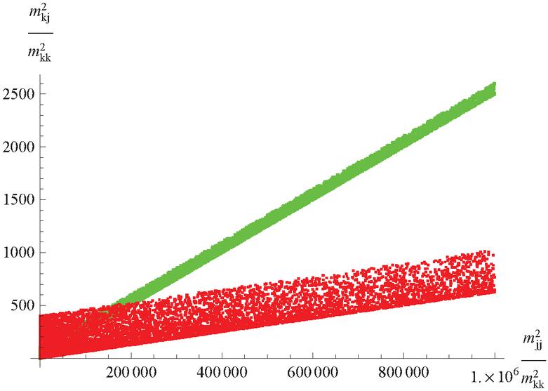
Figure 1 The allowed regions from second constraint for two values of $y$ in case $\left(m_{jj}/m_{kk}\right)\gg 1$. The thinner region correspond to $y=10$ and the other to $y=20$.

For completeness, we turn to the another case where $\left(m_{jj}/m_{kk}\right)$ varies from zero to values of order around one. We show the allowed regions for only one value of $y$ in Figure 2 and for two values of $y$ simultaneously in Figure 3. Opposite to the previous case, the region corresponding to the larger value of the $y$ gets less scattering compared to the one with smaller value of $y$.

Figure 2 The allowed regions from second constraint for one values of $y=0.3$ in the case where $\left(m_{jj}/m_{kk}\right)$ varies from zero to the values of order one.

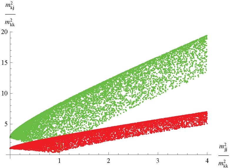
Figure 3 The allowed regions from second constraint for two values of $y$ in the case where $\left(m_{jj}/m_{kk}\right)$ varies from zero to the values of order one. The thinner region correspond to $y=0.5$ and the other one to $y=0.3$.

Now we return to the first constraint equation $y\sin \omega =x$ where $x=m_{ij}/m_{ik}-m_{ik}/m_{ij}$. So the $x$ region is bounded by the two horizontal lines with height$\pm y$. This correspond to the bounded region $(\frac{1}{2}\left(\sqrt{y^2+4}-y\right),\frac{1}{2}\left(\sqrt{y^2+4}+y\right))$ for $m_{ij}/m_{ik}$ as a function $y$. Obviously, the lower bound on $m_{ij}/m_{ik}$ vanishes for large values of $y$ and is the expression is relevant only for smaller values of $y$. Also the upper bound turns out to be $y$ for sufficiently large value of $y$. So we show two regions of allowed values $m_{ij}/m_{ik}$ as a function of $y$ one for small values in Figure 4 and other for large values of $y$ in Figure 5.

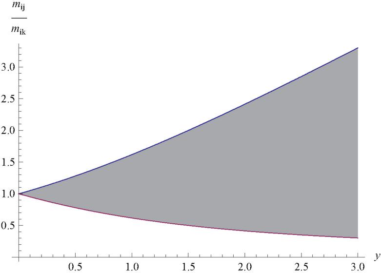
Figure 4 The allowed regions for $\frac{m_{ik}}{m_{ij}}$ as function of $y$ for small values of $y$.

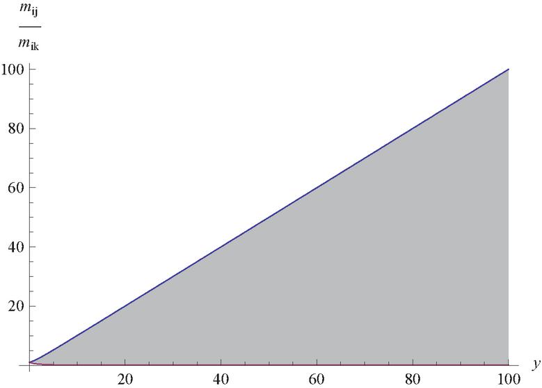
Figure 5 The allowed regions for $\frac{m_{ik}}{m_{ij}}$ as function of $y$ for large values of $y$.

So far we have only discussed the case when $m_{\nu }$ does not have any Majorana phases. What if it does not have the Dirac phase also. It means that one can remove away all the phases in $m_{\nu }$ by rephasing the charged leptons fields. This will provide constraints on the three phases present in $m_{\nu }$. Our formulation provides a different way to attack the problem in the sense that it is able to provide constraints in terms of modulus of mass entries independent of phases. So the condition of vanishing Dirac and Majorana phases in $m_{\nu }$ correspond to the condition $y=0$ in our formulation as already stated earlier in previous section. This implies the following two constraints in terms of modulus of mass entries as

$m_{ik}$	$=$	$m_{ij}$
$m_{jj}$	$=$	$m_{kk}$

Before ending this section, we would like to emphasize again that the indices $i$, $j$ and $k$ can be assigned only three integer values from $1$ to $3$ but only with the condition $i\ne j\ne k$ in all the above equations.

5 Application to Two Texture Zeros

In this section, we discuss a potential application of our formulation in context of neutrino mass matrix with two zero textures. The study of all possible neutrino mass matrices with two zero entries has revealed that only seven such matrices are phenomenologically allowed in light of existing data on neutrino masses and mixing given in Table 1 [14, 15, 16]. At the same time, the three texture zero mass matrices are found to be inconsistent. The question of realization of the two texture zeros in see saw context has been discussed in [24]. The possibility of the origin of textures zeros is GUT scenarios has been addressed in [26, 27]. Another such possibility that has been considered in literature is by invoking some flavour symmetry [28].

The question of Majorana phases in all acceptable neutrino mass matrices with two texture zeros has already been addressed in [21] by studying possible construction of independent measures of CP violation. It has been pointed out that the only one CP measure exist for two textures zeros which can only enter into neutrino oscillations. On the basis, it has been concluded that no Majorana phases are possible in this scenario. However, it is not obvious how the similar conclusion can be realized from a more traditional approach in term of neutrino mixing matrix $U_{PMNS}$. The subject of this section is to explore the possibility of direct realization of the conclusion in the same context.

Table 1 Phenomenologically allowed neutrino mass matrix with two texture zeros in basis where charged lepton mass matrix is real and diagonal

Two Zero Texture Pattern Classification	Texture of $m_{\nu }$	Mass Spectrum
$A_1$	$\left(\begin{array}{ccc}\hfill \mathbf{0}\mathit{\hspace{1em}}\hfill & \hfill \mathbf{0}\mathit{\hspace{1em}}\hfill & \hfill \times \hfill \\ \hfill \mathbf{0}\mathit{\hspace{1em}}\hfill & \hfill \times \mathit{\hspace{1em}}\hfill & \hfill \times \hfill \\ \hfill \times \mathit{\hspace{1em}}\hfill & \hfill \times \mathit{\hspace{1em}}\hfill & \hfill \times \hfill \end{array}\right)$	hierarchical
$A_2$	$\left(\begin{array}{ccc}\hfill \mathbf{0}\mathit{\hspace{1em}}\hfill & \hfill \times \mathit{\hspace{1em}}\hfill & \hfill \mathbf{0}\hfill \\ \hfill \times \mathit{\hspace{1em}}\hfill & \hfill \times \mathit{\hspace{1em}}\hfill & \hfill \times \hfill \\ \hfill \mathbf{0}\mathit{\hspace{1em}}\hfill & \hfill \times \mathit{\hspace{1em}}\hfill & \hfill \times \hfill \end{array}\right)$	hierarchical
$B_1$	$\left(\begin{array}{ccc}\hfill \times \mathit{\hspace{1em}}\hfill & \hfill \times \mathit{\hspace{1em}}\hfill & \hfill \mathbf{0}\hfill \\ \hfill \times \mathit{\hspace{1em}}\hfill & \hfill \mathbf{0}\mathit{\hspace{1em}}\hfill & \hfill \times \hfill \\ \hfill \mathbf{0}\mathit{\hspace{1em}}\hfill & \hfill \times \mathit{\hspace{1em}}\hfill & \hfill \times \hfill \end{array}\right)$	quasi-degenerate
$B_2$	$\left(\begin{array}{ccc}\hfill \times \mathit{\hspace{1em}}\hfill & \hfill \mathbf{0}\mathit{\hspace{1em}}\hfill & \hfill \times \hfill \\ \hfill \mathbf{0}\mathit{\hspace{1em}}\hfill & \hfill \times \mathit{\hspace{1em}}\hfill & \hfill \times \hfill \\ \hfill \times \mathit{\hspace{1em}}\hfill & \hfill \times \mathit{\hspace{1em}}\hfill & \hfill \mathbf{0}\hfill \end{array}\right)$	quasi-degenerate
$B_3$	$\left(\begin{array}{ccc}\hfill \times \mathit{\hspace{1em}}\hfill & \hfill \mathbf{0}\mathit{\hspace{1em}}\hfill & \hfill \times \hfill \\ \hfill \mathbf{0}\mathit{\hspace{1em}}\hfill & \hfill \mathbf{0}\mathit{\hspace{1em}}\hfill & \hfill \times \hfill \\ \hfill \times \mathit{\hspace{1em}}\hfill & \hfill \times \mathit{\hspace{1em}}\hfill & \hfill \times \hfill \end{array}\right)$	quasi-degenerate
$B_4$	$\left(\begin{array}{ccc}\hfill \times \mathit{\hspace{1em}}\hfill & \hfill \times \mathit{\hspace{1em}}\hfill & \hfill \mathbf{0}\hfill \\ \hfill \times \mathit{\hspace{1em}}\hfill & \hfill \times \mathit{\hspace{1em}}\hfill & \hfill \times \hfill \\ \hfill \mathbf{0}\mathit{\hspace{1em}}\hfill & \hfill \times \mathit{\hspace{1em}}\hfill & \hfill \mathbf{0}\hfill \end{array}\right)$	quasi-degenerate
$C$	$\left(\begin{array}{ccc}\hfill \times \mathit{\hspace{1em}}\hfill & \hfill \times \mathit{\hspace{1em}}\hfill & \hfill \times \hfill \\ \hfill \times \mathit{\hspace{1em}}\hfill & \hfill \mathbf{0}\mathit{\hspace{1em}}\hfill & \hfill \times \hfill \\ \hfill \times \mathit{\hspace{1em}}\hfill & \hfill \times \mathit{\hspace{1em}}\hfill & \hfill \mathbf{0}\hfill \end{array}\right)$	quasi-degenerate

Although there are seven such two zero textures, there is possibility that some of them will be related with each other by permutations of indices. So we look for categorizing the seven textures into some classes such that permutations can not take matrices from one class to the one belonging to the other class. However, the matrices in a particular class are related to each other by permutations. A closer inspection of the listed seven textures reveals three such different classes which are grouped as $(A1,A2,B3,B4)$, $(B1,B2)$ and $C$. The matrices in the first two classes are related to the other belonging to the same class as:

$A1\stackrel{\left(2-3\right)}{⟷}A2$	$\stackrel{\left(1-2\right)}{⟷}$	$B4\stackrel{\left(2-3\right)}{⟷}B3$
$B1$	$\stackrel{\left(2-3\right)}{⟷}$	$B2$

So we need to discuss only three matrices representing the three different classes for our purpose simply because our condition of no Majorana phases is blind to the permutations of the indices. Before proceeding further, we need to draw attention on an important issue in this connection. So far we have stated that our two general constraint Equations (25, 26) for all possible combination in $i$, $j$ and k$k$ with condition $i\ne j\ne k$ are equivalent. What we mean by equivalent constraints is that satisfying only one of them is enough to conclude that there is no Majorana phases in the neutrino mass matrix. One does not require simultaneous satisfaction of all possible constraint equations related to each other with permutations. With this clarification, we begin by choosing the three representative matrices for three different classes as $B1$, $B3$ and $C$ and discuss them separately in what follows.

$B1$

For the present texture, we assign the integer value for $j$ as $j=2$. The one of the zero entry corresponding to $m_{22}=0$ in the present case enforces ${\sin }^2\xi$ to vanish from the second constraint equation. Plugging $m_{22}=0$, the two constraint equation turns out to be of following form:

$2y\sin \omega$	$=$	$\left(m_{i2}/m_{ik}-m_{ik}/m_{i2}\right)$	(27)
${\left(m_{k2}/m_{kk}\right)}^2$	$=$	${\displaystyle \frac{1}{4y^2}}$	(28)

If we now assign $k=1$ and $i=3$, the requirement $m_{12}\to 0$ enforces $y$ to take very large value tending to infinity. At the same time, first equation also demands very large value for $y$ to accommodate all possible finite positive values for non-zero elements of $m_{23}$ and $m_{13}$. So both the equation are consistent with the limit $y⟶\mathrm{\infty }$ as $m_{12},m_{22}\to 0$ confirming absence of the Majorana phases in the present texture.

$B3$

In this case, the analysis is not much different with the one discussed above. One need to just assign $k=3$ and $i=1$ in the Equations (27, 28) with the same assignment for $j$ as (2, 2) element is zero for both the cases. One ends up with the same conclusion.

$C$

Here we need to assign $i=3$,$j=1$ and $k=2$ for our purpose. In the limit $m_{22}\to 0$, the two corresponding constraint equations take the following form:

$2y\sin \omega$	$=$	$\left(m_{13}/m_{23}-m_{23}/m_{13}\right)$	(29)
${\displaystyle \frac{{\left(2y{m}_{12}\right)}^2-m_{11}^2}{y^2}}$	$=$	$m_{22}^2$	(30)

Obviously, the requirement that $m_{12}$ and $m_{13}$ can take any finite real positive value demands $y$ to be very large tending to infinity. The second constraint equation, at the same time, is consistent with $y$ tending to infinity in the limit $m_{22}\to 0$. So both the equation are satisfied for the matrix texture leading to no Majorana phases in pattern $C$ also. So have found that all the two zero textures listed in given table are devoid of any Majorana phases.

6 Summary

We have found the conditions in terms of modulus of elements of neutrino mass matrix under which neutrino mass matrix can be diagonalized with $CKM$ type matrix. The allowed regions have been shown for different cases. In addition, we have directly realized that all phenomenologically acceptable neutrino mass textures with two zero entries can be parametrized without introducing any independent Majorana phases.

Thus all such two-zero texture neutrino mass matrices are devoid of independent Majorana Phases. In terms of future scope, our study shows that in three generation two texture zero mass matrix scenario, the only CP violation independent phase source is of Dirac type responsible for CP violation in neutrino oscillation experiments.

References

[1] Q. R. Ahmed et al. (SNO Collaboration), Phys. Rev. Lett. 89, 011301-011302 (2002); Phys. Rev. Lett. 92, 181301 (2004).

[2] S. Fukuda et al. (Super-Kamiokande Collaboration), Phys. Rev. Lett. 86, 5656 (2001); Y. Ashie et al. [Super-Kamiokande Collaboration], Phys. Rev. D 71, 112005 (2005).

[3] K. Eguchi et al. [KamLAND collaboration], Phys. Rev. Lett. 90, 021802 (2003); T. Araki et al. [KamLAND Collaboration], Phys. Rev. Lett. 94, 081801 (2005).

[4] E. Aliu et al. [K2K Collaboration],Phys. Rev. Lett. 94, 081802 (2005).

[5] K. Abe et al. [T2K collaboration], Phys. Rev. Lett. 107, 041801 (2011); P. Adamson et al. [MINOS collaboration], Phys. Rev. Lett. 107, 181802 (2011); Y. Abe et al., [Double Chooz collaboration], Phys. Rev. Lett. 108, 131801 (2012); F. P. An et al., [Daya Bay collaboration], Phys. Rev. Lett. 108, 171803 (2012);Soo-Bong Kim, for RENO collaboration, Phys. Rev. Lett. 108, 191802 (2012).

[6] P. Adamson et al. (NOvA), Phys. Rev. Lett. 118, 231801 (2017); P. F. de Salas, D. V. Forero, C. A. Ternes, M. Tortola, J. W. F. Valle, Phys. Lett. B, 782, 633-640 (2018); I. Esteban, M. C. Gonzalez-Garcia, A. Hernandez-Cabezudo, et al., JHEP 01, 106 (2019).

[7] P. Minkowski, Phys. Lett. B 67, 421 (1977); M. Gell-Mann, P. Ramond and R. Slansky in Supergravity (P. van Niewenhuizen and D. Freedman, eds), (Amsterdam), North Holland, 1979; T. Yanagida in Workshop on Unified Theory and Baryon number in the Universe (O. Sawada and A. Sugamoto, eds), (Japan), KEK 1979; R.N. Mohapatra and G. Senjanovic, Phys. Rev. Lett. 44, 912 (1980);J. Schechter and J.W.F. Valle, Phys. Rev. D 22, 2227 (1980).

[8] M. Fukugita and T. Yanagida, Phys. Lett. B174, 45 (1986).

[9] M.A. Luty, Phys. Rev. D45, 455 (1992); R.N. Mohapatra and X. Zhang, Phys. Rev. D46, 5331 (1992); A. Acker, H. Kikuchi, E. Ma and U. Sarkar, Phys. Rev. D 48, 5006 (1993); M. Flanz, E.A. Paschos and U. Sarkar, Phys. Lett. B 345,248 (1995); M. Flanz, E.A. Paschos, U. Sarkar and J. Weiss, Phys. Lett. B 389, 693 (1996); E. Ma and U. Sarkar, Phys. Rev. Lett. 80, 5716 (1998); T. Hambye, E. Ma and U. Sarkar, Nucl. Phys. B 602, 23 (2001); G. F. Giudice, A. Notari, M. Raidal, A. Riotto and A. Strumia, Nucl. Phys. B 685, 89 (2004); W. Buchmuller, P. Di Bari and M. Plumacher, Nucl. Phys. B 665, 445 (2003); Annals Phys. 315, 305 (2005); W. Buchmuller, R. D. Peccei and T. Yanagida, Ann. Rev. Nucl. Part. Sci. 55, 311 (2005).

[10] Z. Maki, M. Nakagawa and S. Sakata, Prog. Theor. Phys. 28, 870 (1962); B. Pontecorvo, Sov. Phys. JETP 7, 172 (1958) [Zh. Eksp. Teor. Fiz. 34, 247 (1957)]; Sov. Phys. JETP 6, 429 (1957) [Zh. Eksp. Teor. Fiz. 33, 549 (1957)].

[11] B. Kayser, Phys. Rev. D 30 (1984) 1023.

[12] Heidelberg–Moscow Collaboration: H.V. Klapdor-Kleingrothaus et al., Phys. Rev. D 55, 54 (1997); Phys. Lett. B 407, 219 (1997); Phys. Rev. Lett. 83, 41 (1999); Eur. Phys. J. A 12, 147 (2001); Mod. Phys. Lett. A 16, 2409 (2001).

[13] M. Frigerio and A. Y. Smirnov, Nucl. Phys. B 640, 233 (2002); Phys. Rev. D 67, 013007 (2003); A. Merle and W. Rodejohann, Phys. Rev. D 73, 073012 (2006).

[14] P.H. Frampton, S.L. Glashow and D. Marfatia, Phys. Lett. B 536, 79 (2002).

[15] G. C. Branco, R. Gonzalez Felipe, F. R. Joaquim and T. Yanagida, Phys. Lett. B 562, 265 (2003); Z. z. Xing, Phys. Rev. D 69, 013006 (2004); B. C. Chauhan, J. Pulido and M. Picariello, Phys. Rev. D 73, 053003 (2006).

[16] H. Fritzsch, Z. Z. Xing, S. Zhou, JHEP 1109, 083 (2011); D. Meloni, A. Meroni, E. Peinado, Phys. Rev. D 89 (2014) 053009; Shun Zhou, Chin. Phys. C 40 (2016) no.3, 033102; Madan Singh, Gulsheen Ahuja, Manmohan Gupta, Prog. Theor. Exp. Phys. (PTEP) 2016 (12): 123B 08;

[17] X. G. He and A. Zee, Phys. Rev. D 68, 037302 (2003).

[18] S. Kaneko, H. Sawanaka and M. Tanimoto, JHEP 0508, 073 (2005); S. L. Chen, M. Frigerio and E. Ma, Nucl. Phys. B 724, 423 (2005); G. C. Branco, D. Emmanuel-Costa, M. N. Rebelo and P. Roy, Phys. Rev. D 77, 053011 (2008); S. Choubey, W. Rodejohann and P. Roy, Nucl. Phys. B 808, 272 (2009); S. Goswami, S. Khan and A. Watanabe, arXiv:0811.4744 [hep-ph].

[19] C. Jarlskog, Phys. Rev. Lett. 55, 1039 (1985); Z. Phys. C 29, 491 (1985)

[20] J.F. Nieves and P.B. Pal, Phys. Rev. D 36 (1987) 315.

[21] U. Sarkar and S. K. Singh, Nucl. Phys. B 771, 28 (2007).

[22] J. R. Ellis and M. Raidal, Nucl. Phys. B 643 (2002) 229.

[23] G. C. Branco, T. Morozumi, B. M. Nobre and M. N. Rebelo, Nucl. Phys. B 617 (2001) 475; G. C. Branco, R. Gonzalez Felipe, F. R. Joaquim, I. Masina, M. N. Rebelo and C. A. Savoy, Phys. Rev. D 67, 073025 (2003).

[24] A. Kageyama, S. Kaneko, N. Shimoyama and M. Tanimoto, Phys. Lett. B 538, 96 (2002).

[25] S. Kaneko and M. Tanimoto, Phys. Lett. B 551, 127 (2003); S. Kaneko, M. Katsumata and M. Tanimoto, JHEP 0307, 025 (2003).

[26] H. S. Goh, R. N. Mohapatra and S. P. Ng, Phys. Rev. D 68, 115008 (2003).

[27] M. Bando and M. Obara, arXiv:hep-ph/0212242; Prog. Theor. Phys. 109, 995 (2003); M. Bando, S. Kaneko, M. Obara and M. Tanimoto, Phys. Lett. B 580, 229 (2004); arXiv:hep-ph/0405071; S. Dev and S. Kumar,arXiv:0801.2018 [hep-ph].

[28] W. Grimus, A.S. Joshipura, L. Lavoura and M. Tanimoto, Eur. Phys. J C 36, 227 (2004); W. Grimus, PoS (HEP 2005) 186 [hep-ph/0511078]; W. Grimus and L. Lavoura, J. Phys. G 31, 693 (2005); P. H. Frampton, M. C. Oh and T. Yoshikawa, Phys. Rev. D 66, 033007 (2002); M. Hirsch, A. S. Joshipura, S. Kaneko and J. W. F. Valle, Phys. Rev. Lett. 99, 151802 (2007); Di Zhang, Nucl. Phys. B 952,114935(2020); Lu, Jun-Nan and Liu, Xiang-Gan and Ding, Gui-Jun, Phys.Rev.D 101 115020(2020)

Biographies

Hiba Khan is a graduate from Lucknow University, India. She earned M.Sc Degree from Integral University, Lucknow, India. She is currently PhD student in Institute of Engineering & Technology, Lucknow a constituent college of Dr. A. P. J. Abdul Kalam Technical University, Lucknow, Uttar Pradesh. His research interests include the origin of universe, Physics beyond the standard model, theoretical nuclear physics, quantum mechanical neutrino oscillation.

Santosh Kumar Singh is a graduate from Banaras Hindu University, India. He earned M.Sc. Degree in Physics from IIT Bombay, India. He carried out his doctoral thesis work from Physical Research Laboratory (PRL), Ahmedabad, India. He is currently Assistant Professor in Applied Science Department, Institute of Engineering & Technology, Lucknow a constituent college of Dr. A. P. J. Abdul Kalam Technical University, Lucknow, Uttar Pradesh. His research interests include the Neutrino Physics, Physics beyond the standard model, Elementary Particle Physics.

Vivek Kumar Nautiyal is a graduate from Lucknow University, Lucknow, India. He received the M.Tech. degree in applied optics from Indian Institute of Technology Delhi, India in 2014. He has been in constant touch with the nuclear and particle physics for 8 years and earned the Ph.D. degree in physics. He has more than three years of teaching experience in graduation and postgraduation levels. His research interests include the nuclear and particle physics, neutrino physics.

Journal of Graphic Era University, Vol. 10_2, 133–154.
doi: 10.13052/jgeu0975-1416.1025
© 2022 River Publishers

Abstract

1 Introduction

2 Basic Formulation

3 The Constraint Equations

4 The Realization and Understanding of the Constraints

5 Application to Two Texture Zeros

$B1$

$B3$

$C$

6 Summary

References

Biographies