Numerical Forecasting of Covid-19 Epidemic in Odisha Using S.I.R Model: A Case Study
S. Kapoor and Bidisha Jana*
Department of science and Mathematics, Regional Institute of Mathematics (NCERT), Bhubaneswar, Odisha, India
E-mail: janabidisha59@gmail.com
*Corresponding Author
Received 03 January 2022; Accepted 06 February 2022; Publication 07 May 2022
Abstract
In this paper, we study the effectiveness of SIR model (Susceptible- Infected-Removed) in predicting the future development of infectious disease caused by SARS-CoV-2 virus for the Indian state of Odisha. This model helps in checking the effectiveness of controlling measures like lockdown policies and helps in framing new strategies to control the spread of the disease. We formulate a set of differential equations to find the rate of change of susceptible, infected and removed population with respect to time and solve it using Euler’s method. Using the cumulative data of confirmed cases, we try to find the answers to the question of COVID-19 surge. Also, through this we predict the trend in the spread of covid-19 in the state for the next few months. The analysis includes data from March 1 (which is marked as the start of second wave of COVID) to June 28, 2021. We propose predictions on various parameters and factors related to the spread of COVID-19 and on the number of susceptible, infected and removed population until June 2021. By comparing the daily recorded data with the data from our modeling approaches, we conclude that the spread of COVID-19 can be under control in all communities, if proper lockdown restrictions and strong policies are implemented to control the infection rates.
Keywords: SIR model, basic reproduction number, COVID-19, lockdown, herd immunity.
1 Introduction
In the month of December 2019, an infectious disease caused by a novel strand of Coronavirus (SARS-CoV-2) emerged in Wuhan, China. It caused a mild to moderate respiratory syndrome. Aged people especially with underlying medical problems like diabetes, cardiovascular disease, chronic respiratory disease and other illness are more likely to get infected early. The outbreak was announced after one month of the first reported case by World health organization (WHO) on December 31, 2019 and later as pandemic on 11 March, 2020.
The symptoms of the disease are mainly cough, fever and respiratory diseases. The COVID-19 virus spreads mainly through respiratory droplets of saliva or discharge from nose and contact transmission with an incubation period of 2–14 days (Biswas et al., 2020). The spread of the disease is prevented by slowing down the transmission with the help of lockdown and social distancing measures (Telles et al., 2021). Despite of country wide lockdown, it is hard to achieve full control over the transmission of the disease.
India is a country with high population density, where the coronavirus infection (COVID-19) has started from 1 march 2020 followed by a second wave of the disease from February 2021. Because of large population density, the transmission rate or human to human social contact rate is very high in India. The epidemiological data of the disease transmission for Indian state of Odisha has been used to predict the spread of COVID-19 within the state using classical SIR model. The statistical parameters of the disease indicate the high significance of the predicted result. The model includes certain limitations. It does not incorporate uncertainties in the change of infection rate due to change in population structure resulting in the oversimplification of the process. Also, the result is based on limited parameters. But it gives an overall idea of the trend in the spread of infection during the period. Among other Indian states, Maharashtra is worst affected. Odisha has one of the high infection rates comprising a large number of active cases.
The first case of the COVID-19 pandemic was confirmed in this state on 16 March 2020. The state has confirmed 4,07,457 cases, including 42,485 active cases, 3,62,931 recoveries, and 1,988 deaths as of May 2021. Controlling the pandemic has become a challenging problem due to this large number of cases. Mathematical models are employed to study the disease dynamics, identify the influential parameters and access the rapid prevention strategies for reduction in outbreak size. Using the daily reported cases of Odisha, we have estimated the effective reproduction number and make some prediction about the prevalence of the disease for the second wave of covid outbreak from March 1 to June 28. We also study the effect of practices which contribute to the flattening of the curve by reducing the infection rate.
1.1 Modelling of Disease Dynamic
Mathematical models help in analysis of an infectious disease during the course of the outbreak. Application of mathematical model helps to predict the probability of the impact of the disease and help to inform administration and public health care system to mark proper intervention. Some basic assumptions are made while framing the models. Also, the statistical data is used to find the parameters using mathematical operations. These parameters for various infectious diseases are used to calculate the effects of government interventions and impact of policies during the outbreak. The mathematical model helps in deciding the best policies and intervening laws to control the disease and predict its future growth pattern.
Many of the phenomenological models tried to assess and generate short term forecasts with the help of progressive numbers of daily cases based on the reported data (Hojman and Asenjo, 2020). The SIR model is one of the most traditional mathematical models for infectious disease which predict the risk of the pandemic and its outcome in perspective of the future scenario of the disease. Reproduction number (R) is used to indicate the transmission of the infectious disease. The long-used value of R is 1.3 for flu and 2.0 for SARS. In SIR model, infection rate is taken as the time varying constant. As the nationwide lockdown helps reduce face to face contact among peoples, the infection rate also reduces. Value of infection rate helps to observe the overall scenario of coronavirus spreading.
Kermack-Mckendrick in the year 1927 used SIR model for the first time which is used in this work is also the simplest compartmental models. Many works have been undergone during the COVID-19 pandemic using the compartmental model. Many economists have generated a lot of interest to identify the effects and outcomes of current pandemic on economic sectors by exploring different mathematical models which largely includes compartmental models like SIR model along with standard economic models using econometric technique. It has been argued by many economists that most of the controlling parameters which determine the move among compartments are not well structured rather it depends on individual decisions and policies. For example, many of the researchers argued that, the recovery rate and death rate are not just clinical parameters. A large part of it also depends on the decision and policies made by the government and administrating organization. Therefore, these parameters can be used as a function of policy decisions, for example by implementing lockdown and social distancing measures may decrease infection rate and death rate.
1.1.1 Reproduction number
The basic reproduction number measures how transferable the disease is. It is denoted by ‘R’. It calculates the average number of human being that a single infected person transfers the disease to, over the course of infection. The value of basic reproduction number determines the spread of disease. If R 1, then each infected person infects lesser than one person on an average, so the disease will die out. If R 1, then each infected person infects more than one other person on an average and hence the disease will spread. And if R 1, then every infected individual will infect one other individual on average, so the epidemic will occur but there will be neither decrease nor increase in the number of infected populations.
1.1.2 The SIR model
In 1927, A. G. McKendrick and W.O Kermack developed a model in which they divided a fixed population into three groups: susceptible, S(t); infected, I(t); and recovered, R(t). S(t) represents the vulnerable group of individuals or those who are at the risk of getting the infection. I(t) is used to represent those group of population who have been infected with the disease already and are capable of spreading the infection to the susceptible group of population. R(t) denotes the individuals of the population who have been infected before and then removed from the infected category either due to death or due to immunization. These groups of people are not able to transmit the disease to others.
1.2 Objectives and Limitation of the Study
1.2.1 Objective
1. To predict the outcome of the spread of the disease.
2. To manage the disease by taking necessary measures to control it.
3. To make policies and rules in every sector of a country during the epidemic.
4. To make more compartmental models for a better analysis of data from the basic SIR model.
1.2.2 Limitations
1. Computation of SIR model over simplifies the process of predictions for such a complex disease like COVID-19.
2. The model does not include the dormant period between when an individual is exposed to a disease and when that individual becomes infected and contagious.
3. It assumes homogeneous mixing of the population, meaning that all individuals in the population are assumed to have an equal probability of coming in contact with one another. This does not reflect human social structures, in which the majority of contact occurs within limited networks.
4. The SIR model also assumes a closed population with no migration, births, or deaths from causes other than the epidemic.
5. This strategy does not formally quantify the uncertainty in the predictions (Roberto Telles et al., 2021).
2 Methodology
2.1 Epidemiological Model Identification
The SIR model used in pathology demonstrates the relationship between the numbers of individuals susceptible to disease, those presently with the contamination as well as individuals who recovered or died in a population at a particular point of time (Kermack and McKendrick 1927; Hethcote 2000). Statistically, as described below:
Susceptible (S) Infectives (I) Recovered (R)
Where, S number of individuals that are susceptible to COVID-19, I number of individuals infected with COVID19, R number of individuals recovered from COVID-19.
We consider ‘N’ as an overall fixed population inside the affected environment. In SIR model a fixed number of populations is assumed where there is no birth or death by normal reason and only comprise of susceptible individuals, number of infected individuals, number of recovered individuals:
Example N 4.7 crores (Odisha’s population). Input: Estimating the spread of Covid-19 in Odisha data of S(t), I(t) and R(t) for t = t, parameters of , and total population P. Output: Forecast of impending values of S (t), I (t) and R (t). Considering that N is fixed, with no birth or death, makes sense given 120 days; however, it is a generalization. Such a variable may vary over time, so it determines the variable t time in day t 0 at the start of March, 2021.
A two-dimensional structure containing three sets of differential equations with state variables provided as follows:
| (1) | ||
| (2) | ||
| (3) | ||
Where,
For,
Equation (1), refers to the rate of change of the number of susceptible to the disease over time.
Equation (2), refers to the rate of change of the number of infected.
Equation (3), refers to the rate of change of the number of people recovered over time.
Infection Rate ()
An infection rate (or incident rate) is the probability or risk of an infection in a population. It is used to measure the frequency of occurrence of new instances of infection within a population during a specific time period.
The number of infections equals the cases identified in the study or observed.
The “constant or K” is usually an assigned value of 100, 1000, 10000 or 100000, which represents a standard population and time period for interpretation of the rate. Using 100 as the “k” will give an infection rate that may be expressed as a percentage.
Recovery Rate ()
2.2 Probability of Spread of Disease
2.2.1 Ro Basic Reproduction Number (Epidemiological Threshold)
‘R0’ defined as the number of secondary infections caused by a single primary infection; in other words, it determines the number of people infected by contact with a single infected person before his death or recovery.
Table 1 Conditions for the occurrence of pandemic by comparing the value of ‘Ro’
| Epidemic Will Occur If | Epidemic Will Not Occur If |
| The number of infected people increases | The number of infected people decreases |
| is an increasing function | is a decreasing function |
Assumptions
The population size is fixed:
No one enters or leaves the population throughout the duration of the disease i.e., no births, deaths due to other disease, or death by natural causes. Also, the population is confined to a well-defined region.
The population is well mixed/homogeneous mixing:
Ideally, everyone comes in contact with the same fraction of people in each category every day i.e., all individual has an equally likely chance of being infected.
3 Case Scenario
3.1 Status of COVID-19 Situation in Odisha: A Snapshot
The second wave of COVID-19 hit the state of Odisha in March 2021. Of the total number of cases nearly 92% have recovered while less than 8% have remained active. The number of fresh daily cases reported during the first wave remained below 100 for several weeks in Odisha until mid-March this year. The number crossed the 100-mark on March 19 and fresh cases have been steeply rising ever since.
The number of people testing positive jumped from 6,073 on April 27 to 8,386 on April 28. Khordha district was the worst-affected with 1,840 cases, followed by the western districts of Sundargarh and Jharsuguda with 933 and 433 cases., The capital city of Bhubaneswar is located in Khordha district and it has been witnessing a steep rise in cases since it is the gateway to the State. More cases were reported from the State’s western belt when the second wave hit the region in the second half of March.
The situation in many parts of western Odisha was worse in comparison with Bhubaneswar since the former lacked adequate health infrastructure. Reports from the western region indicated that several COVID-19 deaths were not being counted as such in official records. Low level of testing in the interior areas also gave the impression of the number of fresh cases being low.
3.2 Numerical Interpretation
3.2.1 Calculation of Infection Rate and Basic Reproduction Number for Second wave Of Covid Outbreak in Odisha
INFECTION RATE,
1st March, 2021
Total population of Odisha 47,098,218 1 unit
Number of Infected populations (infective) 337,277 0.007 unit
Number of populations at risk (susceptible) 46,760,941 0.993 unit
In percentage, K 100
That is,
BASIC REPRODUCTION NUMBER,
Ro
Infection Period, D 20 (number of days)
Recovery rate,
Therefore, Ro
As, Ro 1.4 1, the disease will spread.
As the value of basic reproduction number is more than one, an infected individual will spread the disease to more than one person and hence the disease will spread among the population and the epidemic will occur.
The value of R0 shows the secondary infection which might change according to the disease dynamic as the time passes. As we see a larger increase in infection rate of covid-19, the value of R0 also increases to 2–3.5 at later stage of infection.
4 Proposed Sir Model Prediction by Euler’s Method
The initial population of susceptible individuals S(to) that helps to identify the future values of discovered infected I(t) discovered recovered R(t) and removed individuals R(t), as shown in Figure 1.
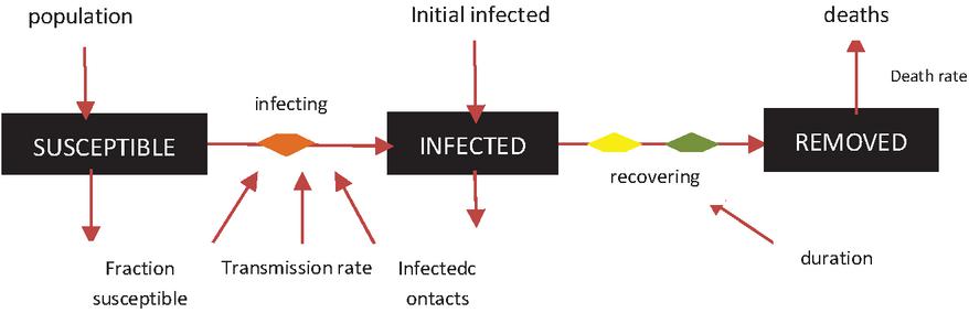
Figure 1 SIR Model prediction for covid-19.
4.1 Numerical Solutions by Euler’s Method
Euler’s method for system of three ordinary differential equations
For , step size , with the initial conditions
The numerical solutions are:
Where,
4.1.1 Euler’s method for SIR model
For , step size , with the initial conditions
not the basic reproduction number)
The numerical solutions are:
First iteration:
Table 2 Populations of S, I, and R compartments from 1 March, 2020 to 28 June, 2020 (120 days)
| Day | Susceptible(S(ti)) | Infective(I(ti)) | Removed(R(ti)) | |
| 0 | 0.993 | 0.007 | 0 | h 1 |
| 1 | 0.9881343000000 | 0.0115157 | 0.00035 | |
| 2 | 0.9801689592890 | 0.018905256 | 0.000925785 | |
| 3 | 0.9671977179183 | 0.030931234 | 0.001871048 | |
| 4 | 0.9462560844618 | 0.050326306 | 0.00341761 | |
| 5 | 0.9129209831541 | 0.081145092 | 0.005933925 | |
| 6 | 0.8610656431094 | 0.128943177 | 0.009991179 | |
| 7 | 0.7833456650767 | 0.200215997 | 0.016438338 | |
| 8 | 0.6735588319413 | 0.29999203 | 0.026449138 | |
| 9 | 0.5321152350430 | 0.426436025 | 0.04144874 | |
| 10 | 0.3732760609416 | 0.563953398 | 0.062770541 | |
| 11 | 0.2259188488218 | 0.68311294 | 0.090968211 | |
| 12 | 0.1178891864456 | 0.756986956 | 0.125123858 | |
| 13 | 0.0554207829913 | 0.781606011 | 0.162973206 | |
| 14 | 0.0250987309909 | 0.772847763 | 0.202053506 | |
| 15 | 0.0115204823233 | 0.747783623 | 0.240695894 | |
| 16 | 0.0054901027130 | 0.716424822 | 0.278085075 | |
| 17 | 0.0027368306125 | 0.683356853 | 0.313906317 | |
| 18 | 0.0014276682446 | 0.650498173 | 0.348074159 | |
| 19 | 0.0007775813357 | 0.618623351 | 0.380599068 | |
| 20 | 0.0004408603557 | 0.588028904 | 0.411530235 | |
| 21 | 0.0002593933134 | 0.558808926 | 0.440931681 | |
| 22 | 0.0001579274042 | 0.530969946 | 0.468872127 | |
| 23 | 0.0000992291105 | 0.504480147 | 0.495420624 | |
| 24 | 0.0000641877292 | 0.479291181 | 0.520644632 | |
| 25 | 0.0000426525004 | 0.455348157 | 0.544609191 | |
| 26 | 0.0000290572842 | 0.432594344 | 0.567376598 | |
| 27 | 0.0000202582724 | 0.410973426 | 0.589006316 | |
| 28 | 0.0000144303443 | 0.390430583 | 0.609554987 | |
| 29 | 0.0000104865109 | 0.370912997 | 0.629076516 | |
| 30 | 0.0000077638027 | 0.35237007 | 0.647622166 | |
| 31 | 0.0000058487905 | 0.334753482 | 0.665240669 | |
| 32 | 0.0000044782584 | 0.318017178 | 0.681978344 | |
| 33 | 0.0000034813442 | 0.302117316 | 0.697879202 | |
| 34 | 0.0000027451022 | 0.287012187 | 0.712985068 | |
| 35 | 0.0000021935877 | 0.272662129 | 0.727335678 | |
| 36 | 0.0000017749119 | 0.259029441 | 0.740968784 | |
| 37 | 0.0000014530838 | 0.246078291 | 0.753920256 | |
| Day | Susceptible(S(ti)) | Infective(I(ti)) | Removed(R(ti)) | |
| 38 | 0.0000012027831 | 0.233774627 | 0.766224171 | |
| 39 | 0.0000010059570 | 0.222086092 | 0.777912902 | |
| 40 | 0.0000008495707 | 0.210981944 | 0.789017207 | |
| 41 | 0.0000007240998 | 0.200432972 | 0.799566304 | |
| 42 | 0.0000006225064 | 0.190411425 | 0.809587952 | |
| 43 | 0.0000005395338 | 0.180890937 | 0.819108524 | |
| 44 | 0.0000004712160 | 0.171846458 | 0.82815307 | |
| 45 | 0.0000004145323 | 0.163254192 | 0.836745393 | |
| 46 | 0.0000003671604 | 0.15509153 | 0.844908103 | |
| 47 | 0.0000003272999 | 0.147336993 | 0.852662679 | |
| 48 | 0.0000002935436 | 0.139970177 | 0.860029529 | |
| 49 | 0.0000002647824 | 0.132971697 | 0.867028038 | |
| 50 | 0.0000002401364 | 0.126323137 | 0.873676623 | |
| 51 | 0.0000002189021 | 0.120007001 | 0.87999278 | |
| 52 | 0.0000002005132 | 0.11400667 | 0.88599313 | |
| 53 | 0.0000001845113 | 0.108306352 | 0.891693463 | |
| 54 | 0.0000001705227 | 0.102891049 | 0.897108781 | |
| 55 | 0.0000001582410 | 0.097746508 | 0.902253333 | |
| 56 | 0.0000001474138 | 0.092859194 | 0.907140659 | |
| 57 | 0.0000001378317 | 0.088216244 | 0.911783618 | |
| 58 | 0.0000001293204 | 0.08380544 | 0.916194431 | |
| 59 | 0.0000001217339 | 0.079615176 | 0.920384703 | |
| 60 | 0.0000001149496 | 0.075634424 | 0.924365461 | |
| 61 | 0.0000001088637 | 0.071852709 | 0.928147183 | |
| 62 | 0.0000001033882 | 0.068260079 | 0.931739818 | |
| 63 | 0.0000000984481 | 0.06484708 | 0.935152822 | |
| 64 | 0.0000000939793 | 0.06160473 | 0.938395176 | |
| 65 | 0.0000000899266 | 0.058524498 | 0.941475412 | |
| 66 | 0.0000000862425 | 0.055598276 | 0.944401637 | |
| 67 | 0.0000000828861 | 0.052818366 | 0.947181551 | |
| 68 | 0.0000000798215 | 0.050177451 | 0.949822469 | |
| 69 | 0.0000000770179 | 0.047668581 | 0.952331342 | |
| 70 | 0.0000000744479 | 0.045285155 | 0.954714771 | |
| 71 | 0.0000000720880 | 0.043020899 | 0.956979029 | |
| 72 | 0.0000000699171 | 0.040869856 | 0.959130074 | |
| 73 | 0.0000000679168 | 0.038826366 | 0.961173567 | |
| 74 | 0.0000000660709 | 0.036885049 | 0.963114885 | |
| 75 | 0.0000000643650 | 0.035040798 | 0.964959137 | |
| Day | Susceptible(S(ti)) | Infective(I(ti)) | Removed(R(ti)) | |
| 76 | 0.0000000627862 | 0.03328876 | 0.966711177 | |
| 77 | 0.0000000613232 | 0.031624324 | 0.968375615 | |
| 78 | 0.0000000599657 | 0.030043109 | 0.969956831 | |
| 79 | 0.0000000587046 | 0.028540955 | 0.971458987 | |
| 80 | 0.0000000575318 | 0.027113908 | 0.972886035 | |
| 81 | 0.0000000564398 | 0.025758214 | 0.97424173 | |
| 82 | 0.0000000554222 | 0.024470304 | 0.975529641 | |
| 83 | 0.0000000544728 | 0.02324679 | 0.976753156 | |
| 84 | 0.0000000535864 | 0.022084451 | 0.977915495 | |
| 85 | 0.0000000527580 | 0.020980229 | 0.979019718 | |
| 86 | 0.0000000519832 | 0.019931219 | 0.980068729 | |
| 87 | 0.0000000512579 | 0.018934659 | 0.98106529 | |
| 88 | 0.0000000505785 | 0.017987926 | 0.982012023 | |
| 89 | 0.0000000499417 | 0.017088531 | 0.982911419 | |
| 90 | 0.0000000493443 | 0.016234105 | 0.983765846 | |
| 91 | 0.0000000487835 | 0.0154224 | 0.984577551 | |
| 92 | 0.0000000482569 | 0.014651281 | 0.985348671 | |
| 93 | 0.0000000477620 | 0.013918717 | 0.986081235 | |
| 94 | 0.0000000472966 | 0.013222782 | 0.986777171 | |
| 95 | 0.0000000468588 | 0.012561643 | 0.98743831 | |
| 96 | 0.0000000464468 | 0.011933561 | 0.988066392 | |
| 97 | 0.0000000460588 | 0.011336884 | 0.98866307 | |
| 98 | 0.0000000456933 | 0.01077004 | 0.989229915 | |
| 99 | 0.0000000453488 | 0.010231538 | 0.989768417 | |
| 100 | 0.0000000450240 | 0.009719962 | 0.990279993 | |
| 101 | 0.0000000447177 | 0.009233964 | 0.990765992 | |
| 102 | 0.0000000444286 | 0.008772266 | 0.99122769 | |
| 103 | 0.0000000441558 | 0.008333653 | 0.991666303 | |
| 104 | 0.0000000438982 | 0.00791697 | 0.992082986 | |
| 105 | 0.0000000436550 | 0.007521122 | 0.992478834 | |
| 106 | 0.0000000434251 | 0.007145066 | 0.99285489 | |
| 107 | 0.0000000432079 | 0.006787813 | 0.993212144 | |
| 108 | 0.0000000430026 | 0.006448423 | 0.993551534 | |
| 109 | 0.0000000428085 | 0.006126002 | 0.993873955 | |
| 110 | 0.0000000426249 | 0.005819702 | 0.994180255 | |
| 111 | 0.0000000424513 | 0.005528717 | 0.994471241 | |
| 112 | 0.0000000422870 | 0.005252281 | 0.994747676 | |
| 113 | 0.0000000421315 | 0.004989667 | 0.99501029 | |
| 114 | 0.0000000419844 | 0.004740184 | 0.995259774 | |
| 115 | 0.0000000418451 | 0.004503175 | 0.995496783 | |
| 116 | 0.0000000417132 | 0.004278016 | 0.995721942 | |
| 117 | 0.0000000415883 | 0.004064116 | 0.995935843 | |
| 118 | 0.0000000414699 | 0.00386091 | 0.996139048 | |
| 119 | 0.0000000413579 | 0.003667865 | 0.996332094 | |
| 120 | 0.0000000412517 | 0.003484472 | 0.996515487 |
5 Imposement of Lockdown in Odisha
Odisha announced a state wide lockdown from May 5 to May 19 which was then extended to june1 and then to June 17.
It is very difficult to get control over COVID-19 through one-day voluntary Janata Curfew and social distancing. Therefore, there was a need to take some hard steps. Lockdown is the most appropriate decision as a preventive measure. Odisha responded with lots of effective mitigation measures in order to fight against the pandemic. It took proactive steps to set mass vaccination target. Odisha strengthened its health care system and used its disaster management expertise to get control over the spread of the virus. Many states of the country decided to implement lockdown in their states to control the COVID-19. The infection rate reduced from 0.7–0.8 to 0.2–0.3 during the lockdown which caused the flattening of the curve of infected population.
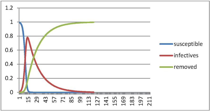
Figure 2 Forecasting of time-dependent SIR model of SARS-CoV-2 in Odisha from March to June 2021.
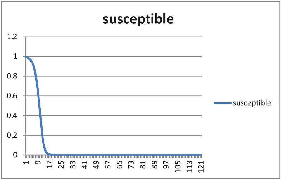
Figure 3 Forecasting of SIR model for susceptible individuals of SARS-CoV-2 in Odisha.
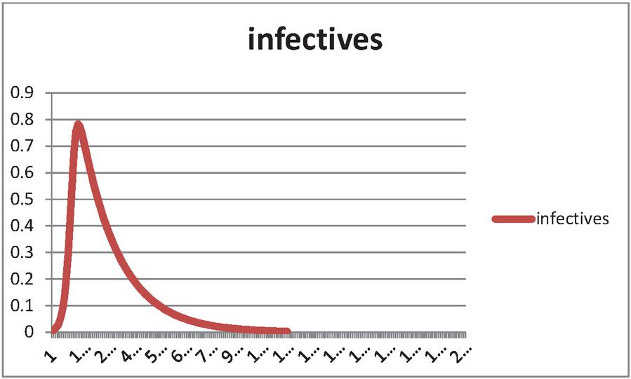
Figure 4 Forecasting of time-dependent SIR model of infected cases of SARS-CoV-2 in Odisha.
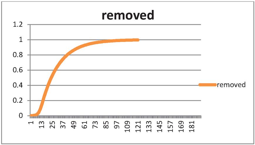
Figure 5 Forecasting of time-dependent SIR model of removed cases of SARS-CoV-2 in Odisha.
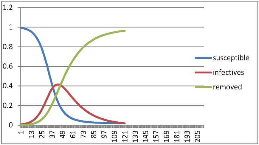
Figure 6 Flatten curve of SIR model of SARS-CoV-2 in Odisha from March to June 2021 (actual scenario).
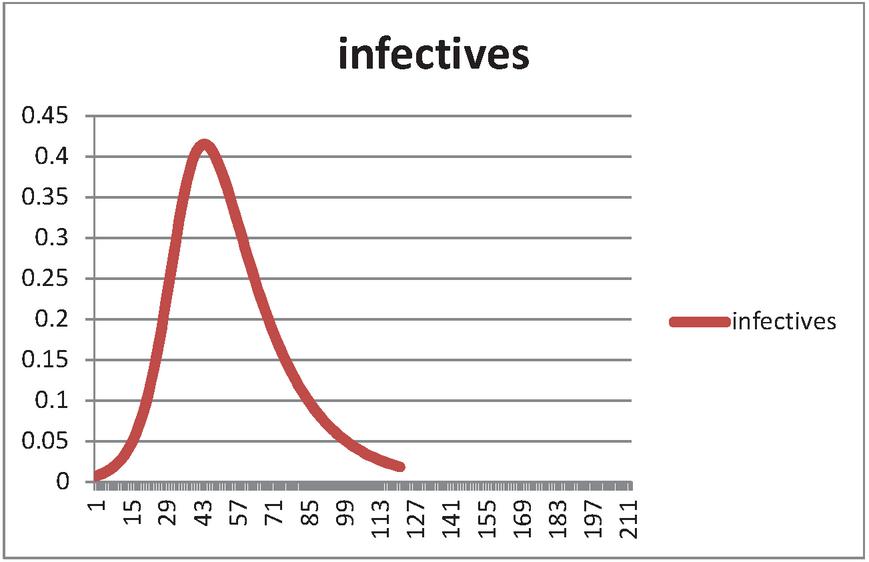
Figure 7 Flatten graph curve of active infected during the lockdown period.
6 Result
The graphical representation of the SIR model is explained below: Figure 3 explains the susceptible cases of SARS-CoV-2. Around 4 crore people are susceptible during the initial time of outburst, and future values are predicted in upcoming days. The predicted result is shown using graphical representation which shows the case scenario if there were no lockdowns (Figure 2). The flattened graph in Figure 7 shows the reduction in infection rate due to imposition of lockdown. The Infected individuals crossed nearly 8,83490 in the June month. The people that recovered from the infection are shown in Figure 5. The recovery rate is continuously the other of the transmittable period. The dying rate is predicted by the number of infected individual’s multiple with the death rate and infected duration. The susceptible fraction value is decided by susceptible population. Figure 2 explains the predicted result of spread of SARS-CoV-2 in odisha from the start date of second wave until June month in odisha in absence of lockdown. The difference in the graph can be easily marked by comparing the peak of the infection curve of both the figures i.e. Figures 2 and 6. without a lockdown, the infection curve attains it’s peak earlier while the same peak in Figure 6 is delayed and lower. Both predicted and the original results of the confirmed, infected, and removed values are compared through graphical representations.
7 Conclusion
In this paper, we proposed an SIR model with a flatten curve and herd immunity based on a susceptible population that reduce over time due to spread of infection causing a difference in infected and removed population. It is advisable to encourage the implementation of lockdown policies to avoid massive contamination of the population. Strict adequate measures must be enforced to still prevent and manage the spread of COVID-19. Many countries have produced significant steps to scale back the number of infected citizens, like lock-down measures, awareness program generated through media, sanitization campaigns to hamper the spread of the disease. Additional measures like early detection approaches, isolation of susceptible individuals to stop mixing them with no-symptoms and self-quarantine individuals, traffic restrictions, and medical treatment helps to stop the rise in the number of infected individuals. Strong lockdown policies are required to be implemented. Our simulation results show the amount of susceptible, infected, and recovered persons, and also, the transmission rate and deathrate concerning time tracks the outburst of SARS-CoV-2 in Odisha. The effects of lockdown and herd immunity reduce the spread of transmission. By adopting herd immunity and the effective measures, the number of susceptible individuals can be decreased. There are numerous limitations of this model because the SIR model used here is that the simplest one and predictions that begin won’t be accurate enough; sometimes, it also depends on the published data and their constancy. Necessary public health policies have to be implemented in state with a high spread of COVID-19 cases as early as possible to manage its spread. Different mathematical models can be worked out for the epidemiological model to improve the prediction results further.
References
Bagal, D., Rath, A., Barua, A., and Patnaik, D. (2021). Estimating the parameters of susceptible-infected-recovered model of COVID-19 cases in India during lockdown periods. Retrieved 27 August 2021, from https://pubmed.ncbi.nlm.nih.gov/32834642/.
Biswas, S., Ghosh, J., Sarkar, S., and Ghosh, U. (2020). COVID-19 pandemic in India: a mathematical model study. Nonlinear Dynamics, 102(1), 537–553. https://doi.org/10.1007/s11071-020-05958-z
CDRI Report (2020). Response to COVID-19: Odisha, India. www.cdri.world/casestudy/response-tocovid19-by-odisha.pdf.
COVID-19: Odisha State Dashboard. State Dashboard. (2021). Retrieved 4 September 2021, from https://statedashboard.odisha.gov.in/.
Cooper, I., Mondal, A., and Antonopoulos, C. (2021). A SIR model assumption for the spread of COVID-19 in different communities. Retrieved 27 August 2021, from https://www.ncbi.nlm.nih.gov/pmc/articles/PMC7321055/.
Carcione, J., Santos, J., Bagaini, C., and Ba, J. (2021). A Simulation of a COVID-19 Epidemic Based on a Deterministic SEIR Model. Retrieved 26 August 2021, from https://www.frontiersin.org/articles/10.3389/fpubh.2020.00230/full.
Garikipati N (2020).Odisha’s quiet success in warfare on Covid-19 pandemic. Coverage Circle. https://www.policycircle.org/life/odishas-quiet-success-in-war-on-covid
Hojman, S., and Asenjo, F. (2020). Phenomenological dynamics of COVID-19 pandemic: Meta-analysis for adjustment parameters. Chaos: An Interdisciplinary Journal Of Nonlinear Science, 30(10), 103120. https://doi.org/10.1063/5.0019742
Infection rate – Wikipedia. (2021). Retrieved 9 September 2021, from https://en.wikipedia.org/wiki/Infection\_rate
Kumar M, Ghosh S (2020).Using lessons from disaster management, Odisha takes on Covid-19. MONGABAY. https://india.mongabay.com/2020/04/using-lessons-from-disaster-management-odisha-takes-on-covid-19/
Kumar S, Maheshwari V, Prabhu J, Prasanna M et al (2020). Social economic impact of COVID-19 outbreak in India. Int J Pervasive Compute Common 16(4):309–319. https://doi.org/10.1108/IJPCC-06-2020-0053
Kwok OK, Lai F et al. (2020). Herd immunity–estimating the level required to halt the COVID-19 epidemics in affected countries. J Infect 80(6):32–33. https://doi.org/10.1016/j.jinf.2020.03.027
Mathematical modelling of infectious disease - Wikipedia. En.wikipedia.org. (2021). Retrieved 27 August 2021, from https://en.wikipedia.org/wiki/Mathematical\_modelling\_of\_infectious\_disease.
Mohanty D (2020).How the Covid-19 pandemic unfolded in Odisha. Hindustan Times. www.hindustantimes.com/india-news/how-the-covid-19-pandemic-unfolded-in-odisha/story-HVv0Y5KB1mGXiP1TiKrHI.html
Mukesh Jahar, P.K. Ahluwalia and Ashok Kumar. (2020). COVID-19 Epidemic Forecast in Different States of India using SIR Model. Retrieved 27 August 2021, from https://www.medrxiv.org/content/10.1101/2020.05.14.20101725v1.full.pdf.
Pani MB (2020).No End to COVID-19 containment woes for residents of Katapali in Odisha. The New Indian Express. www.newindianexpress.com/states/odisha/2020/jul/30/no-end-to-covid-19-containment-woes-for-residents-of-katapali-in-odisha-2176649.html.
Pal M (2020).Empower gram panchayats to be able to deal with crises like COVID-19 effectively in rural areas. National Herald.. www.nationalheraldindia.com/india/empower-gram-panchayats-to-beable-to-deal-with-crises-like-covid-19-effectively-in-rural-areas
Riyapan, P., Shuaib, S., and Intarasit, A. (2021). A Mathematical Model of COVID-19 Pandemic: A Case Study of Bangkok, Thailand. Retrieved 25 August 2021, from https://www.hindawi.com/journals/cmmm/2021/6664483/.
Roberto Telles, C., Lopes, H., and Franco, D. (2021). SARS-COV-2: SIR Model Limitations and Predictive Constraints. Symmetry, 13(4), 676. https://doi.org/10.3390/sym13040676
Telles, C., Roy, A., Ajmal, M., Mustafa, S., Ahmad, M., and de la Serna, J. et al. (2021). The Impact of COVID-19 Management Policies Tailored to Airborne SARS-CoV-2 Transmission: Policy Analysis. JMIR Public Health And Surveillance, 7(4), e20699. https://doi.org/10.2196/20699
Tiwari, V., Deyal, N., and Bisht, N. (2021). Mathematical Modeling Based Study and Prediction of COVID-19 Epidemic Dissemination Under the Impact of Lockdown in India. Retrieved 25 August 2021, from https://www.frontiersin.org/articles/10.3389/fphy.2020.586899/full.
Zaman, G., Jung, I., Torres, D., and Zeb, A. (2021). Mathematical Modeling and Control of Infectious Diseases. Retrieved 23 August 2021, from https://www.hindawi.com/journals/cmmm/2017/7149154/.
Biographies

S. Kapoor is an Assistant professor of Mathematics at the Regional Institute of Education, Bhubaneswar. He has completed his Ph.D. in Mathematics from IIT Roorkee. His area of specialization is computational Fluid Dynamics, Hydrodynamics stability of flow through porous media, Applied numerical method, FEM, B- Spline FEM, SEM, SCM, Numerical solution of PDE.

Bidisha Jana is a student of Mathematics. She has completed her B.Sc(mathematics).B.Ed from Regional Institute of Education, Bhubaneswar. She is currently pursuing M.Sc. in Mathematics at Assam University, Silchar.
Journal of Graphic Era University, Vol. 10_2, 95–116.
doi: 10.13052/jgeu0975-1416.1023
© 2022 River Publishers